Fixed Effects + DID
library(ggdag)
library(tidyverse)
library(broom)
library(fixest)
library(gapminder)

# set seed
set.seed(1990)
The fixed effects DAG
Say we wanted to estimate the effect of GDP on life expectancy, and had a DAG like the following:
dagify(Life ~ GDP + Geography + Population + Pollution + WW2 + Equator,
       GDP ~ Geography + Population + Pollution + WW2 + Equator,
       exposure = "GDP", outcome = "Life") %>%
  ggdag_status(text = FALSE, use_labels = "name") + theme_dag(legend.position = "none")
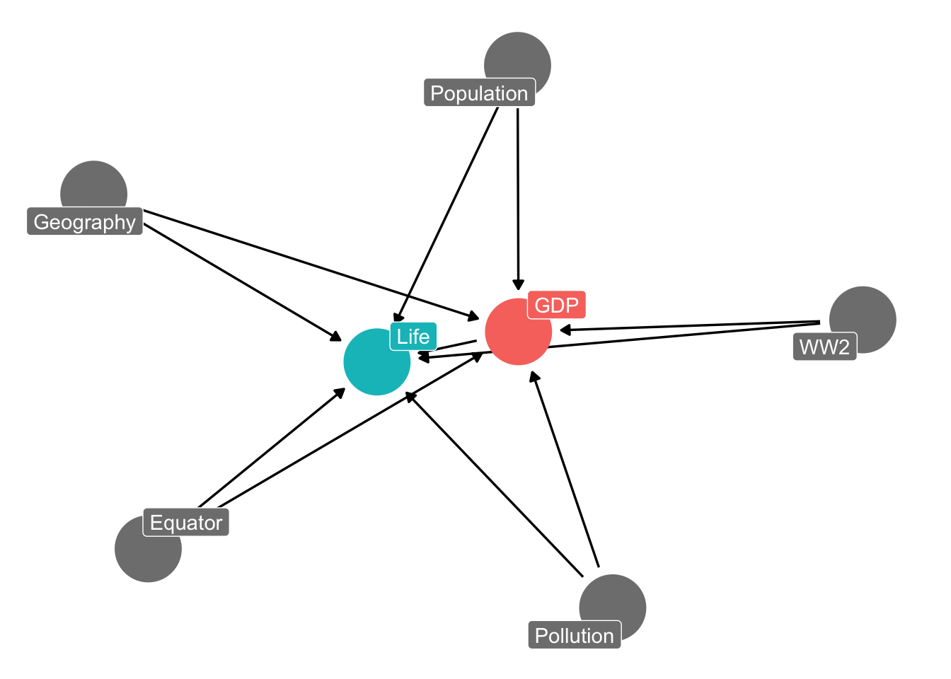
The key thing here is that some of these variables only vary across countries, but not within them. They are constant within the country. For example, a country’s distance from the equator is fixed. Same with whether or not they participated in WW2. Other variables also vary within country, like a country’s level of pollution (or population) which changes over time.
The insight is that we can think about all of the variables that are constant within country as a general “country” backdoor. The “country” backdoor is all of the differences between the countries in our data that are static or fixed. Pollution and population are not included because they also vary within country.
dagify(Life ~ GDP + Country + Population + Pollution,
       GDP ~ Country + Population + Pollution,
       exposure = "GDP", outcome = "Life") %>%
  ggdag_status(text = FALSE, use_labels = "name") + theme_dag(legend.position = "none")
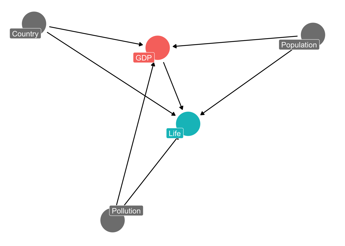
We can use fixed effects to control for the “country” backdoor, and implicitly, all variables that are static within countries.
Here’s the naive regression, without country fixed effects:
# naive
m1 = lm(lifeExp ~ gdpPercap + pop, data = gapminder)
tidy(m1)
## # A tibble: 3 × 5
##   term        estimate     std.error statistic   p.value
##   <chr>          <dbl>         <dbl>     <dbl>     <dbl>
## 1 (Intercept)  5.36e+1 0.322            166.   0
## 2 gdpPercap    7.68e-4 0.0000257         29.9  4.04e-158
## 3 pop          9.73e-9 0.00000000238      4.08 4.72e-  5
Here’s the fixed effect regression, using the fixest package. The general template is: feols(Y ~ X1 + X2 + ... | UNIT, data = DATA)
# naive
m2 = feols(lifeExp ~ gdpPercap + pop | country, data = gapminder)
tidy(m2)
## # A tibble: 2 × 5
##   term          estimate    std.error statistic  p.value
##   <chr>            <dbl>        <dbl>     <dbl>    <dbl>
## 1 gdpPercap 0.000394     0.000177          2.22 0.0279
## 2 pop       0.0000000620 0.0000000180      3.44 0.000776
Notice how the estimate on GDP changes with the addition of FE. Notice also that we still haven’t closed all the backdoors in our original DAG! Pollution is a backdoor, and varies within country, so the country fixed effect will not suffice. We need to control for it, but we have no data on it! This captures the broad takeaway of FE:
- FE help us close backdoors that are constant within the unit
- But we still need to control for confounds that vary within the unit (e.g., population, pollution)
- We can add those alongside FE (e.g., population)
- but sometimes we don’t have data on all confounds that vary within unit, so we’re not out of the woods (e.g., pollution)
Simulation to show how it works
We’re gonna make up some data to estimate effect of a teacher having an MA on their student’s test scores. The DAG looks like this:
# draw the dag
dag = dagify(score ~ teacher_ma + male + parent_income,
       teacher_ma ~ male + parent_income,
       exposure = "teacher_ma", outcome = "score")

ggdag_status(dag, text = FALSE, use_labels = "name") + theme_dag()
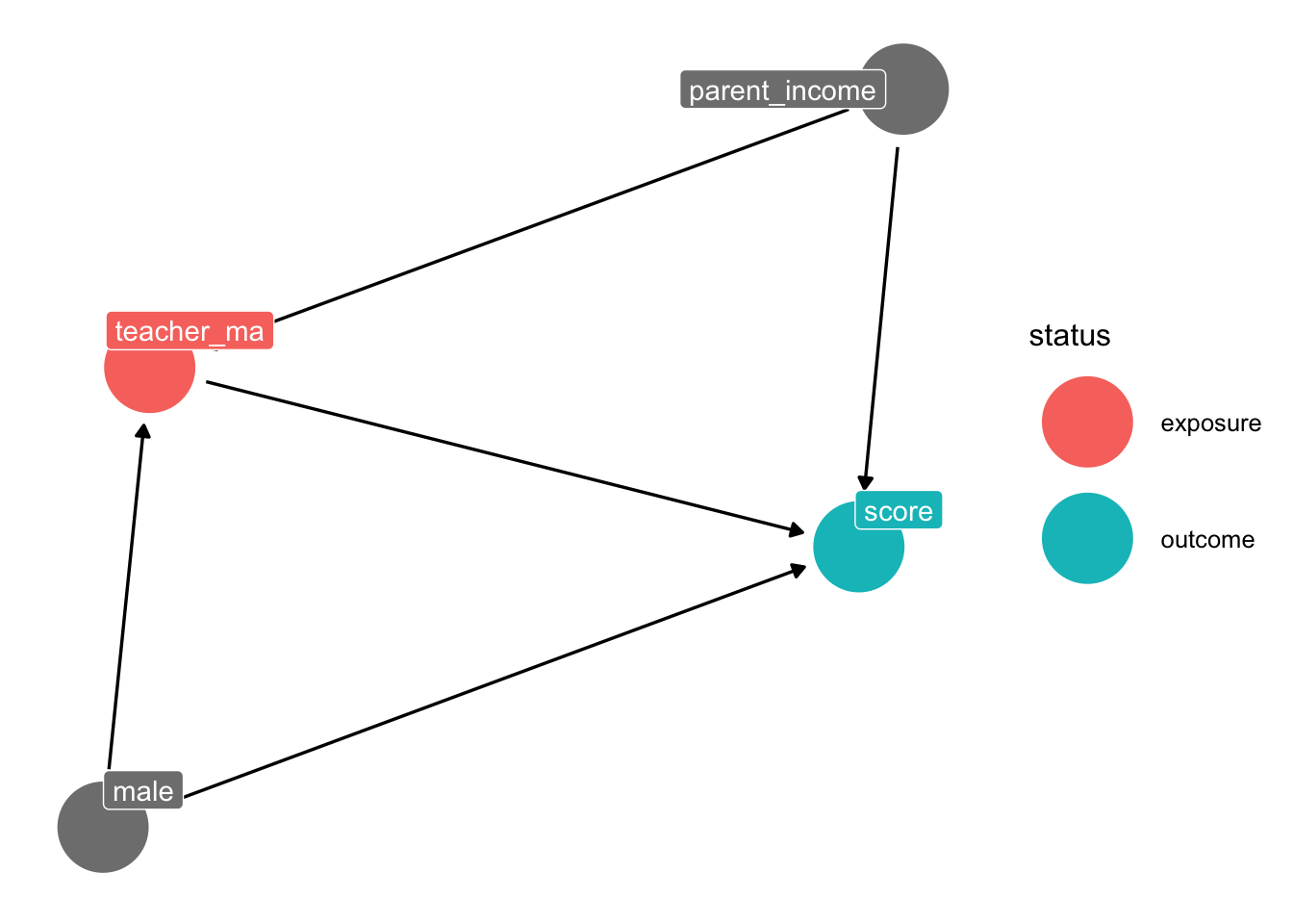
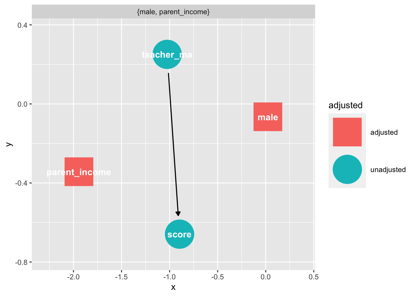
Notice we have some backdoors that we need to control for:
ggdag_adjustment_set(dag)
Let’s make up the data:
# make up student data
kids = tibble(student = c("Joe", "Jessica", "Laia", "Jeff", "Martin"),
       male = sample(c(1, 0), size = 5, replace = TRUE),
       parent_income = rnorm(5))


fake = crossing(student = unique(kids$student),
         test = 1:50) %>%
  left_join(kids) %>%
  mutate(teacher_ma = 2*male + 3*parent_income + rnorm(250)) %>%
  mutate(score = 5*teacher_ma + -2*male + 5*parent_income + rnorm(250))
Notice above that the true effect of teacher_ma on score is 5.
Here’s the (wrong) result when we don’t control for anything:
# naive regression
lm(score ~ teacher_ma, data = fake) %>% tidy()
## # A tibble: 2 × 5
##   term        estimate std.error statistic   p.value
##   <chr>          <dbl>     <dbl>     <dbl>     <dbl>
## 1 (Intercept)    -2.30    0.144      -16.0 5.30e- 40
## 2 teacher_ma      5.22    0.0639      81.6 3.12e-181
Here’s the (right) result when we control for all confounds:
# correctly specify controls
lm(score ~ teacher_ma + parent_income + male, data = fake) %>% tidy()
## # A tibble: 4 × 5
##   term          estimate std.error statistic   p.value
##   <chr>            <dbl>     <dbl>     <dbl>     <dbl>
## 1 (Intercept)      0.264    0.154       1.72 8.72e-  2
## 2 teacher_ma       5.03     0.0628     80.1  3.04e-178
## 3 parent_income    4.79     0.310      15.4  4.98e- 38
## 4 male            -2.39     0.210     -11.4  1.74e- 24
Here’s the (right) result when we use student FE:
# use fixed effects to account for student-constant variables
feols(score ~ teacher_ma | student, data = fake) %>% tidy()
## # A tibble: 1 × 5
##   term       estimate std.error statistic      p.value
##   <chr>         <dbl>     <dbl>     <dbl>        <dbl>
## 1 teacher_ma     5.04    0.0444      113. 0.0000000362
Notice above how we get the right answer even without controlling for the parent_income and male backdoors. This is because we are implicitly controlling for them.
Diff-in-diff by hand
Remember in class we were looking at the effect of Pokemon Go on exercise using difference-in-differences. Let’s see how this works by making up some data where we already know the effect of the app on exercise (let’s set the effect to 2).
set.seed(1990)
#Create our data
fake_pokemon =
  tibble(year = sample(2002:2010,10000,replace=T),
         app = sample(c("Has app", "Doesn't have app"), 10000, replace = TRUE)) %>%
  mutate(after = ifelse(year > 2007, 1, 0)) %>%
  mutate(D = after*(app == "Has app")) %>%
  mutate(Y = 2*D + .25*year + (app == 'Has app') +  rnorm(10000))
We can find that exact difference by filling out the 2x2 before/after treatment/control table:
| Before 2016 | After 2016 | ∆ | |
|---|---|---|---|
| Doesn’t have app | A | B | B − A |
| Has app | C | D | D − C |
| ∆ | C − A | D − B | (D − C) − (B − A) |
Here’s the table in our data:
#Now, get before-after differences for both groups
means = fake_pokemon %>% group_by(app,after) %>% summarize(Y=mean(Y))
means %>% pivot_wider(names_from = "after", values_from = "Y") %>%
  rename(After = `1`, Before = `0`)
## # A tibble: 2 × 3
## # Groups:   app [2]
##   app              Before After
##   <chr>             <dbl> <dbl>
## 1 Doesn't have app   501.  502.
## 2 Has app            502.  505.
Let’s calculate all of the differences we need. Here’s B - A:
502 - 501
## [1] 1
This is the change in exercise in the pre to post-period among those who didn’t receive treatment (i.e., download the app). The exercise among these kids increased by 1. Why? Remember, all sorts of thing are happening in the world at any given time. And the app was released in summer! So this increase might just be because kids are out of school, or its nicer out, etc.
Let’s calculate D - C:
505 - 502
## [1] 3
This is the change in exercise in the pre to post-period among those who did receive treatment (i.e., downloaded the app). The exercise among these kids increased by 3. Is this increase causal? No! Notice above that exercise also went up a bit among students who didn’t even have the app. So exercise went up over this time (because school’s out, it’s nice out, etc.). We need to remove this general increase in exercise. Let’s get the diff-in-diff estimate:
(505 - 502) - (502 - 501)
## [1] 2
The diff-in-diff estimate is that exercise went up by 2 as a result of Pokemon Go.
Diff-in-diff with regression
We can also do diff-in-diff via regression (in fact this is how everyone does it). The basic template is: lm(Y ~ TREATMENT + TIME + TREATMENT*TIME, data = DATA)
Yis our outcome of interest (here: exercise)TREATMENTis a variable that tells us an observation’s treatment status (here: has pokemon go vs. doesn’t have it)TIMEis a variable that tells us if an observation is pre- or post-treatment (here: has pokemon go been released yet?)TREATMENT*TIMEis the interaction of these two variables (more on this later)
m1 = lm(Y ~ app + after + app*after, data = fake_pokemon)
tidy(m1)
## # A tibble: 4 × 5
##   term             estimate std.error statistic   p.value
##   <chr>               <dbl>     <dbl>     <dbl>     <dbl>
## 1 (Intercept)        501.      0.0184   27233.  0
## 2 appHas app           1.01    0.0259      39.0 1.44e-309
## 3 after                1.13    0.0321      35.2 8.69e-256
## 4 appHas app:after     1.99    0.0452      43.9 0
The coefficient for the interaction term (appHas app:after) is our diff-in-diff estimate. Here we would say that Pokemon Go increased the exercise rate by 2 among app users.