Tidy data
Tidy data
We can use the pivot_longer function to make data that is in “wide” format into “long” format.
Here’s an example, using the drinks dataset from fivethirtyheight.
# load libraries
library(tidyverse)
library(fivethirtyeight)

# too many countries, let's look at a few
# %in% is a new logical operator: returns observations that match one of the strings
drinks_subset =
  drinks %>%
  filter(country %in% c("USA", "China", "Italy", "Saudi Arabia"))


# let's gather the three alcohol variables into two: type and serving
tidy_drinks = drinks_subset %>%
  pivot_longer(cols = c(beer_servings, spirit_servings, wine_servings),
               names_to = "type", values_to = "serving")
tidy_drinks
## # A tibble: 12 × 4
##    country      total_litres_of_pure_alcohol type            serving
##    <chr>                               <dbl> <chr>             <int>
##  1 China                                 5   beer_servings        79
##  2 China                                 5   spirit_servings     192
##  3 China                                 5   wine_servings         8
##  4 Italy                                 6.5 beer_servings        85
##  5 Italy                                 6.5 spirit_servings      42
##  6 Italy                                 6.5 wine_servings       237
##  7 Saudi Arabia                          0.1 beer_servings         0
##  8 Saudi Arabia                          0.1 spirit_servings       5
##  9 Saudi Arabia                          0.1 wine_servings         0
## 10 USA                                   8.7 beer_servings       249
## 11 USA                                   8.7 spirit_servings     158
## 12 USA                                   8.7 wine_servings        84
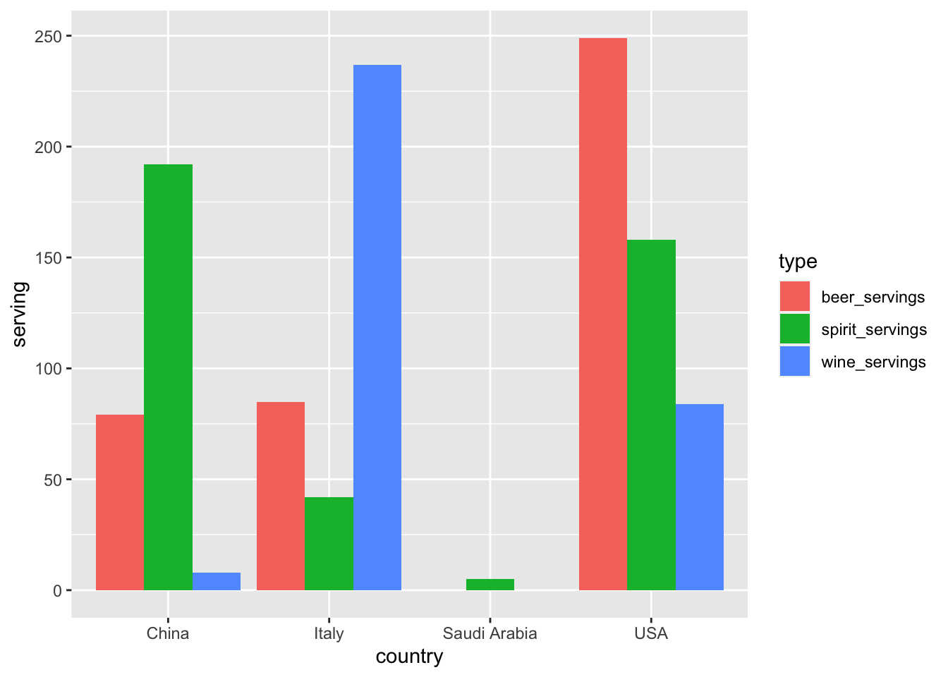
# let's put position = dodge in geom_col, which will place bars side by side
ggplot(tidy_drinks, aes(x = country, y = serving, fill = type)) +
  geom_col(position = "dodge")
Here’s another example, using the masculinity survey from fivethirtyeight.
# different dataset on masculinity
masculinity_survey
## # A tibble: 189 × 12
##    question  response overall age_18_34 age_35_64 age_65_over white_yes white_no
##    <fct>     <fct>      <dbl>     <dbl>     <dbl>       <dbl>     <dbl>    <dbl>
##  1 "In gene… Very ma…    0.37      0.29      0.42        0.37      0.34     0.44
##  2 "In gene… Somewha…    0.46      0.47      0.46        0.47      0.5      0.39
##  3 "In gene… Not ver…    0.11      0.13      0.09        0.13      0.11     0.11
##  4 "In gene… Not at …    0.05      0.1       0.02        0.03      0.04     0.06
##  5 "In gene… No answ…    0.01      0         0.01        0.01      0.01     0
##  6 "How imp… Very im…    0.16      0.18      0.17        0.13      0.11     0.26
##  7 "How imp… Somewha…    0.37      0.38      0.37        0.32      0.38     0.35
##  8 "How imp… Not too…    0.28      0.18      0.31        0.37      0.32     0.2
##  9 "How imp… Not at …    0.18      0.26      0.15        0.18      0.18     0.19
## 10 "How imp… No answ…    0         0         0.01        0         0        0
## # ℹ 179 more rows
## # ℹ 4 more variables: children_yes <dbl>, children_no <dbl>,
## #   straight_yes <dbl>, straight_no <dbl>
# focus on one question
# collapse age categories into long format
manly_pressure = masculinity_survey %>%
  filter(question == "Do you think that society puts pressure on men in a way that is unhealthy or bad for them?") %>%
  pivot_longer(names_to = "ages",
               values_to = "percent",
               c(age_18_34, age_35_64, age_65_over))

manly_pressure
## # A tibble: 9 × 11
##   question          response overall white_yes white_no children_yes children_no
##   <fct>             <fct>      <dbl>     <dbl>    <dbl>        <dbl>       <dbl>
## 1 Do you think tha… Yes         0.6       0.58     0.65         0.56        0.66
## 2 Do you think tha… Yes         0.6       0.58     0.65         0.56        0.66
## 3 Do you think tha… Yes         0.6       0.58     0.65         0.56        0.66
## 4 Do you think tha… No          0.39      0.41     0.35         0.44        0.34
## 5 Do you think tha… No          0.39      0.41     0.35         0.44        0.34
## 6 Do you think tha… No          0.39      0.41     0.35         0.44        0.34
## 7 Do you think tha… No answ…    0.01      0.01     0            0.01        0
## 8 Do you think tha… No answ…    0.01      0.01     0            0.01        0
## 9 Do you think tha… No answ…    0.01      0.01     0            0.01        0
## # ℹ 4 more variables: straight_yes <dbl>, straight_no <dbl>, ages <chr>,
## #   percent <dbl>
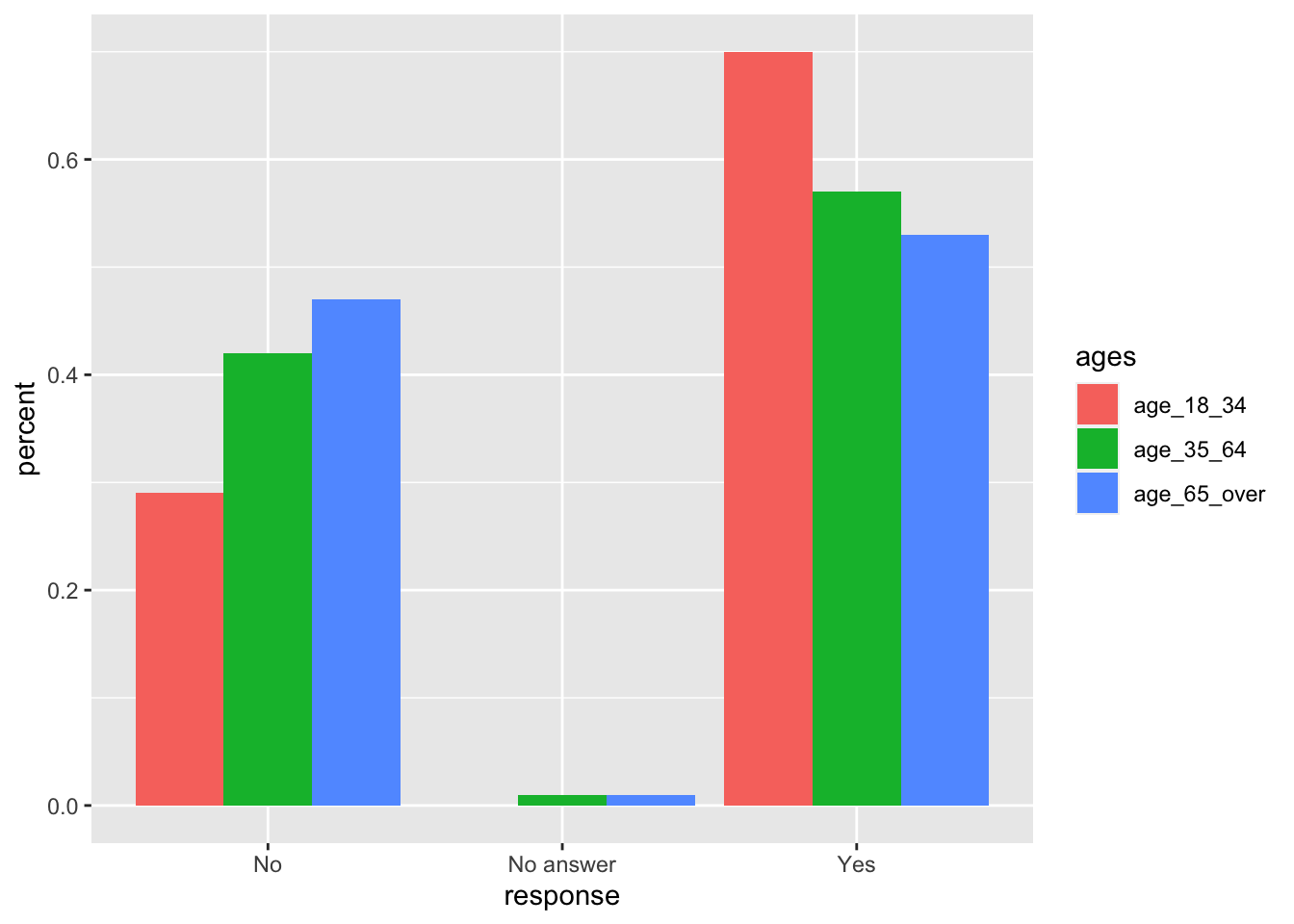
And we can plot the results:
# plot
ggplot(manly_pressure, aes(x = response, y = percent, fill = ages)) +
  geom_col(position = "dodge")
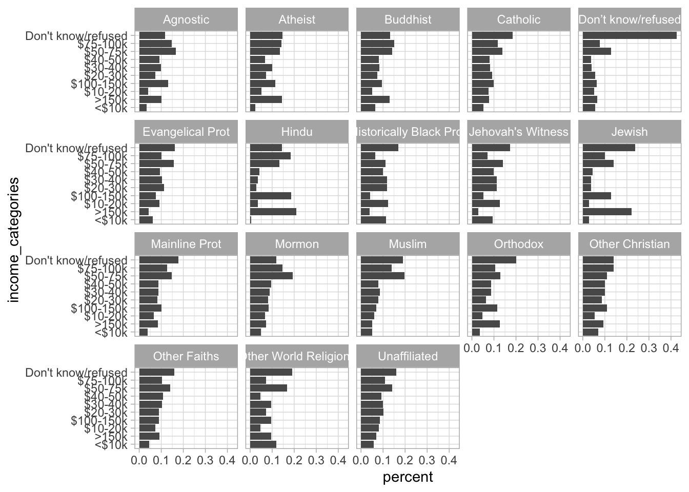
Finally, here’s another example using relig_income. Notice here how instead of explicitly writing out every variable we want to collapse, we can just exclude the only other variable in the dataset via the “-”.
# look at the data
relig_income
## # A tibble: 18 × 11
##    religion `<$10k` `$10-20k` `$20-30k` `$30-40k` `$40-50k` `$50-75k` `$75-100k`
##    <chr>      <dbl>     <dbl>     <dbl>     <dbl>     <dbl>     <dbl>      <dbl>
##  1 Agnostic      27        34        60        81        76       137        122
##  2 Atheist       12        27        37        52        35        70         73
##  3 Buddhist      27        21        30        34        33        58         62
##  4 Catholic     418       617       732       670       638      1116        949
##  5 Don’t k…      15        14        15        11        10        35         21
##  6 Evangel…     575       869      1064       982       881      1486        949
##  7 Hindu          1         9         7         9        11        34         47
##  8 Histori…     228       244       236       238       197       223        131
##  9 Jehovah…      20        27        24        24        21        30         15
## 10 Jewish        19        19        25        25        30        95         69
## 11 Mainlin…     289       495       619       655       651      1107        939
## 12 Mormon        29        40        48        51        56       112         85
## 13 Muslim         6         7         9        10         9        23         16
## 14 Orthodox      13        17        23        32        32        47         38
## 15 Other C…       9         7        11        13        13        14         18
## 16 Other F…      20        33        40        46        49        63         46
## 17 Other W…       5         2         3         4         2         7          3
## 18 Unaffil…     217       299       374       365       341       528        407
## # ℹ 3 more variables: `$100-150k` <dbl>, `>150k` <dbl>,
## #   `Don't know/refused` <dbl>
# make tidy
tidy_relig = relig_income %>%
  pivot_longer(-religion, names_to = "income_categories",
               values_to = "responses") %>%
  group_by(religion) %>%
  mutate(percent = responses/sum(responses))


# make the plot
ggplot(tidy_relig, aes(x = income_categories, y = percent)) +
  geom_col() +
  facet_wrap(vars(religion)) +
  coord_flip() +
  theme_light()
Counts and percentages (group_by + tally)
Say we wanted to count how many characters in the starwars dataset have blonde, brown, etc., hair. I can do this with group_by and tally:
starwars %>%
  group_by(hair_color) %>%
  tally()
## # A tibble: 13 × 2
##    hair_color        n
##    <chr>         <int>
##  1 auburn            1
##  2 auburn, grey      1
##  3 auburn, white     1
##  4 black            13
##  5 blond             3
##  6 blonde            1
##  7 brown            18
##  8 brown, grey       1
##  9 grey              1
## 10 none             37
## 11 unknown           1
## 12 white             4
## 13 <NA>              5
Or, with group_by and summarise and n():
starwars %>%
  group_by(hair_color) %>%
  summarise(n = n())
## # A tibble: 13 × 2
##    hair_color        n
##    <chr>         <int>
##  1 auburn            1
##  2 auburn, grey      1
##  3 auburn, white     1
##  4 black            13
##  5 blond             3
##  6 blonde            1
##  7 brown            18
##  8 brown, grey       1
##  9 grey              1
## 10 none             37
## 11 unknown           1
## 12 white             4
## 13 <NA>              5
Now, say I wanted to calculate the percent of characters with each eye color. I can do this below:
starwars %>%
  group_by(hair_color) %>%
  tally() %>%
  mutate(percent = n/sum(n))
## # A tibble: 13 × 3
##    hair_color        n percent
##    <chr>         <int>   <dbl>
##  1 auburn            1  0.0115
##  2 auburn, grey      1  0.0115
##  3 auburn, white     1  0.0115
##  4 black            13  0.149
##  5 blond             3  0.0345
##  6 blonde            1  0.0115
##  7 brown            18  0.207
##  8 brown, grey       1  0.0115
##  9 grey              1  0.0115
## 10 none             37  0.425
## 11 unknown           1  0.0115
## 12 white             4  0.0460
## 13 <NA>              5  0.0575
Factor variables
Sometimes we have a categorical variable (e.g., months of the year) that we understand as having some qualitative ordering (e.g., January comes before June). R doesn’t know this though, but we can tell it using factor variables.
Here’s an example using some data I made up:
# i have data on weather that looks like this:
weather = tibble(temp = c(80, 23, 14, 23, 25),
                 month = c("January", "December",
                           "July", "June", "October"))

weather
## # A tibble: 5 × 2
##    temp month
##   <dbl> <chr>
## 1    80 January
## 2    23 December
## 3    14 July
## 4    23 June
## 5    25 October
# i want the month variable in order
# i can use factors for this
weather_factor = weather %>%
  mutate(month_factor = factor(month, levels = c("January", "June",
                                          "July", "October",
                                          "December")))
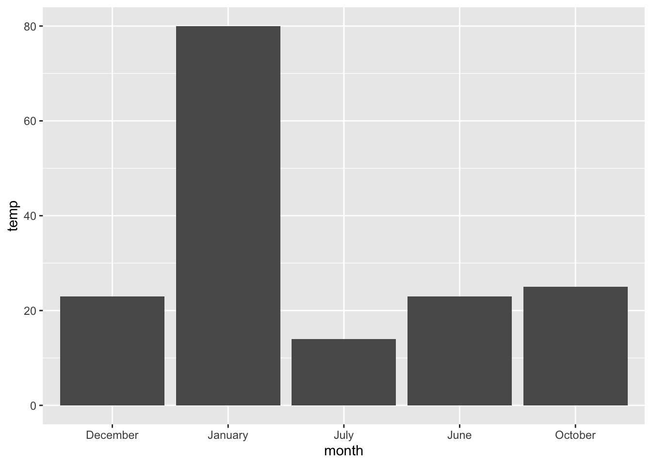
Notice plot without factor:
ggplot(weather, aes(x = month, y = temp)) + geom_col()
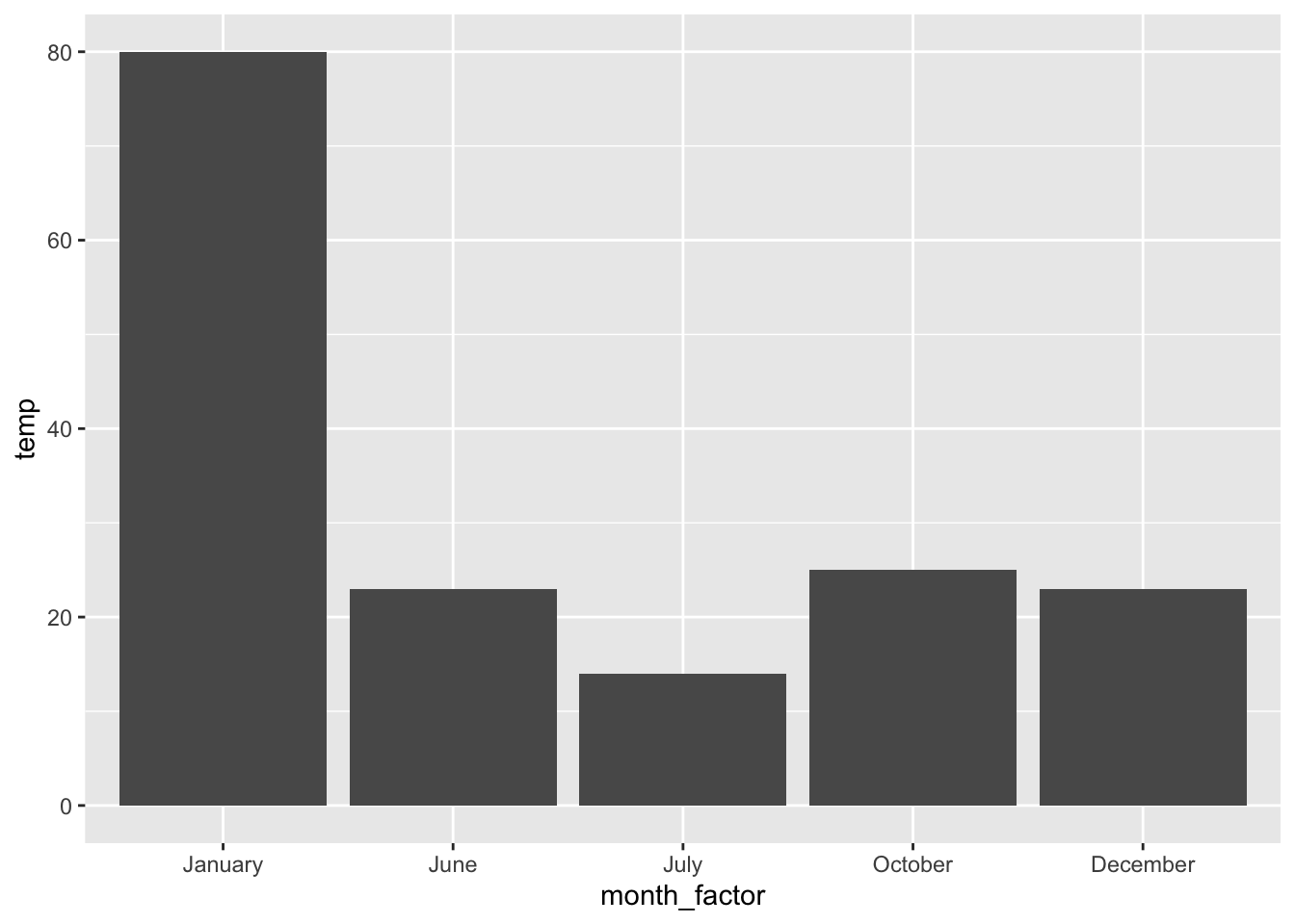
And new and imrpoved plot where month is a factor:
ggplot(weather_factor, aes(x = month_factor, y = temp)) + geom_col()
fct_reorder
Instead of explicitly telling R how we want to order a factor, we can instead use another variable in the dataset to determine the order.
Look at the example below, using the starwars dataset:
# starwars example
starwars
## # A tibble: 87 × 14
##    name     height  mass hair_color skin_color eye_color birth_year sex   gender
##    <chr>     <int> <dbl> <chr>      <chr>      <chr>          <dbl> <chr> <chr>
##  1 Luke Sk…    172    77 blond      fair       blue            19   male  mascu…
##  2 C-3PO       167    75 <NA>       gold       yellow         112   none  mascu…
##  3 R2-D2        96    32 <NA>       white, bl… red             33   none  mascu…
##  4 Darth V…    202   136 none       white      yellow          41.9 male  mascu…
##  5 Leia Or…    150    49 brown      light      brown           19   fema… femin…
##  6 Owen La…    178   120 brown, gr… light      blue            52   male  mascu…
##  7 Beru Wh…    165    75 brown      light      blue            47   fema… femin…
##  8 R5-D4        97    32 <NA>       white, red red             NA   none  mascu…
##  9 Biggs D…    183    84 black      light      brown           24   male  mascu…
## 10 Obi-Wan…    182    77 auburn, w… fair       blue-gray       57   male  mascu…
## # ℹ 77 more rows
## # ℹ 5 more variables: homeworld <chr>, species <chr>, films <list>,
## #   vehicles <list>, starships <list>
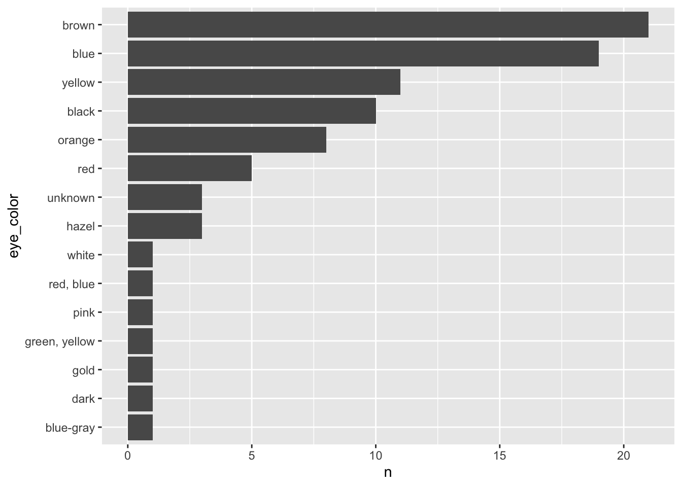
# count how many characters with each eye_color
star_eyes = starwars %>%
  group_by(eye_color) %>%
  tally()

star_eyes = star_eyes %>%
  mutate(eye_color = fct_reorder(eye_color, n))

ggplot(star_eyes, aes(x = eye_color, y = n)) +
  geom_col() +
  coord_flip()