Confounds
Confounding
Remember that we’re always trying to estimate the effect of some treatment, X, on some outcome, Y. The problem is that simply looking at the relationship between X and Y can lead you astray, since lots of things are correlated in the world that have no causal relationship (e.g., number of shark attacks and amount of ice cream consumed are probably positively correlated; but obviously ice cream does not cause shark attacks!).
This “being led astray” by data is what we call confounding. What we want to do in this part of the class is use causal models to figure out how to estimate the effect of X on Y, and avoid confounding.
Marriage, divorce, age, and confounding
Remember in class that we can have a DAG like the below, where the age (A) at which people get married has a negative causal effect on the marriage (M) rate (places where people wait till later to get married have lower marriage rates) and a negative causal effect on the divorce (D) rate (places where people wait to get married have lower divorce rates).
library(ggdag)
library(tidyverse)
library(broom)
set.seed(1990)

dagify(D ~ A,
       M ~ A) %>%
  ggdag(layout = "circle") +
  theme_dag()
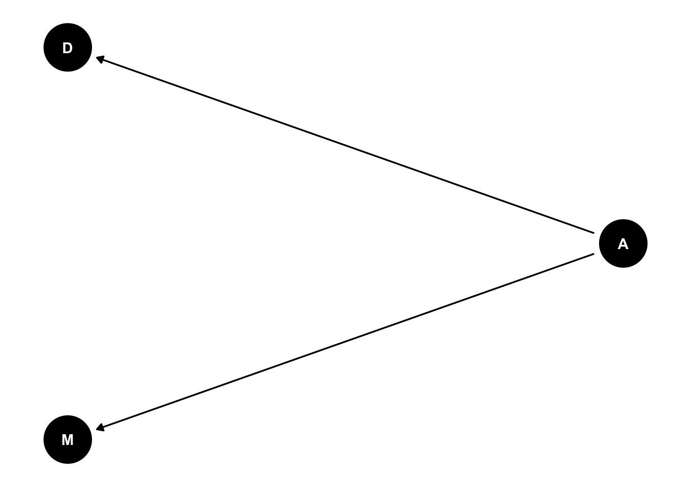
Note that there is no arrow from marriage rate (M) to divorce (D). We have explicitly made our data so that there is no causal effect of M on D. And yet! this DAG will produce data that shows a strong relationship between M and D.
Faking some data helps us see this:
fake = tibble(age = rnorm(100),
       marriage = -2*age + rnorm(100),
       divorce = -2*age + rnorm(100))

ggplot(fake, aes(x = marriage, y = divorce)) +
  geom_point() + geom_smooth(method = "lm") +
  theme_light()
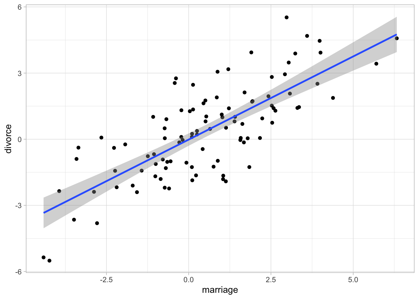
We end up with a confounded estimate of the effect of marriage on divorce.
Backdoors and front-doors
The reason that the above DAG produces a confounded estimate of marriage on divorce is that there is a backdoor path from marriage to divorce, going through age. A backdoor path is a path linking our X and Y variables in a non-causal way. If we don’t close backdoor paths, our estimate of the effect of X (marriage) on Y (divorce) will be confounded. To close the backdoor path we must control for age.
Front-door paths are the ways in which X causes Y. They might be direct (as in an arrow from X to Y), or indirect, as in an arrow from X, to Z, to Y. We want to keep front doors open and not accidentally control for them.
The experimental gold standard
Remember that in an experiment, we randomize assignment to some treatment, measure an outcome we care about, and compare whether the units that got the treatment have better or worse results on the outcome than the group that didn’t get the treatment.
We can simulate a fake experiment (on rats) using R:
rats = tibble(rat_id = 1:200,
              vaccine = sample(c(1, 0), size = 200,
                               replace = TRUE),
              social = sample(c(1, 0), size = 200,
                               replace = TRUE)) %>%
  mutate(covid_levels = -2*vaccine + 3*social + rnorm(200))

rats
## # A tibble: 200 × 4
##    rat_id vaccine social covid_levels
##     <int>   <dbl>  <dbl>        <dbl>
##  1      1       1      0       -2.35
##  2      2       0      1        3.74
##  3      3       1      0        1.38
##  4      4       1      0       -1.82
##  5      5       1      1        1.90
##  6      6       1      1        2.15
##  7      7       1      0       -1.60
##  8      8       1      1        0.923
##  9      9       1      0       -2.90
## 10     10       0      1        4.34
## # ℹ 190 more rows
Note that in making up our data, we decided that the vaccine would have an effect of -2 on covid_levels.
We can estimate the effect of the vaccine on COVID using regression:
# estimate treatment effect
m1 = lm(covid_levels ~ vaccine, data = rats)
tidy(m1)
## # A tibble: 2 × 5
##   term        estimate std.error statistic  p.value
##   <chr>          <dbl>     <dbl>     <dbl>    <dbl>
## 1 (Intercept)     1.56     0.181      8.64 1.89e-15
## 2 vaccine        -2.06     0.250     -8.26 2.05e-14
Note the estimated coefficient on the vaccine is pretty close to the true effect (-2). The reason is because there is no backdoor path, no third variable, or set of variables, causing both the vaccine and COVID levels.
Easy DAGs
Remember, unless otherwise specified, when we are looking at DAGs we assume that X is the treatment variable and Y is the outcome variable.
dag = dagify(Y ~ X)
ggdag(dag) + theme_dag_blank()
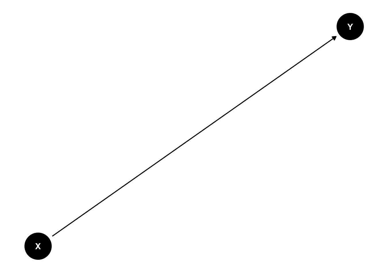
No need to close anything here.
dag = dagify(Y ~ X + B + A + C + G,
             B ~ A + C,
             G ~ C)
ggdag(dag) + theme_dag_blank()
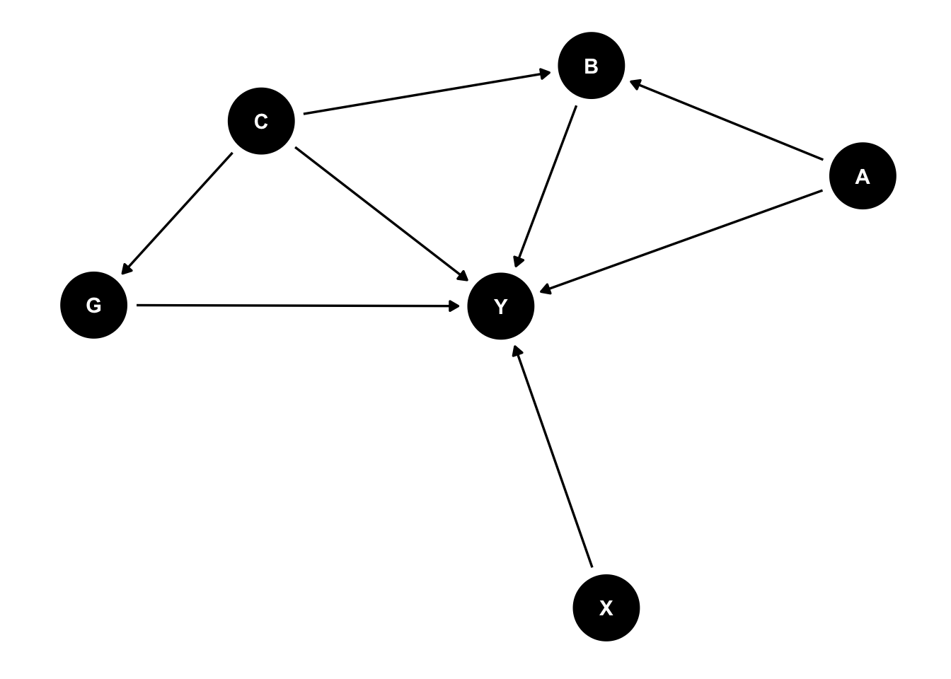
No need to close anything here either. All we care about is estimating the effect of X on Y; it doesn’t matter that other things also cause Y!
When things go wrong: Elemental confounds
We talked about three common scenarios in which confounding can take place: forks, pipes, and colliders.
forks
Remember, the fork looks like this:
confounder_triangle(x = "Has Huge beard",
                    y = "Amount of basketball watched",
                    z = "Love James Harden") %>%
  ggdag(use_labels = "label") +
  theme_dag()
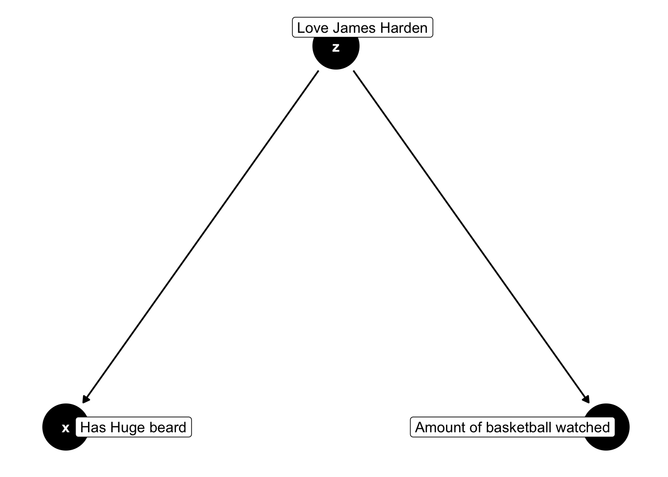
Need to control for loving James harden!
Or like this:
confounder_triangle(x = "Marriage rate",
                    y = "Divorce rate",
                    z = "Median age at marriage", x_y_associated = TRUE) %>%
  ggdag(use_labels = "label") +
  theme_dag()
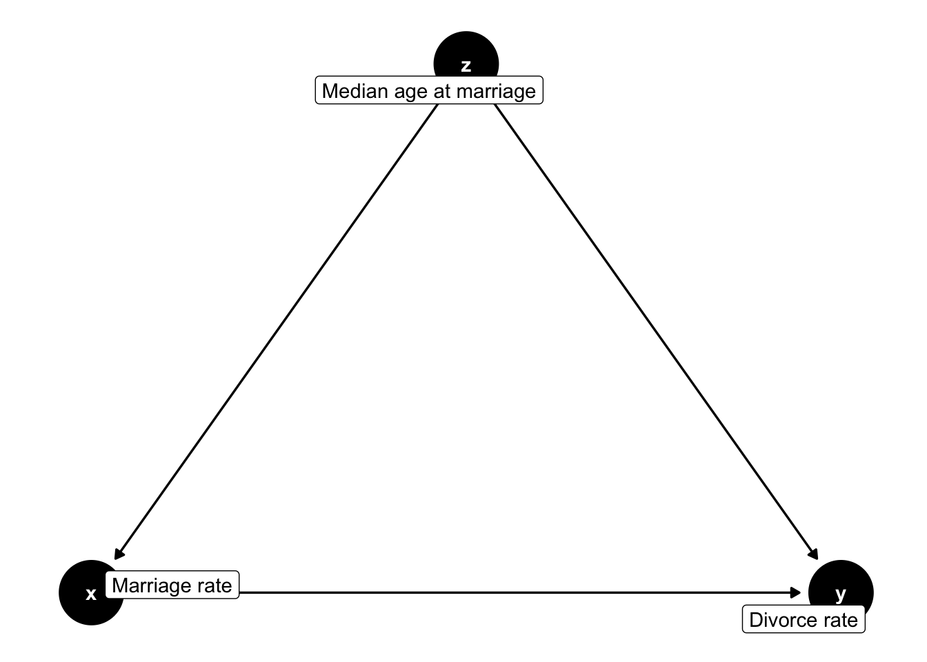
Need to control for median age at marriage!
pipes
The pipe looks like this and it’s an example of why we shouldn’t close front-door paths:
dagify(Y ~ B + G,
       B ~ X,
       labels = c("Y" = "Plant growth",
                  "B" = "Good bacteria",
                  "G" = "Starting size",
                  "X" = "Fertilizer")) %>%
  ggdag(use_labels = "label") +
  theme_dag_blank()
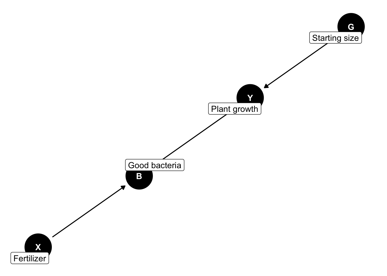
If we control for presence of good bacteria we are closing front-door from Fertilizer to Plant Growth (which is bad)!
collider
The collider looks like this:
collider_triangle(x = "Qualtiy research",
                  y = "Surprising results",
                  m = "Published") %>%
  ggdag(use_labels = "label") +
  theme_dag_blank()
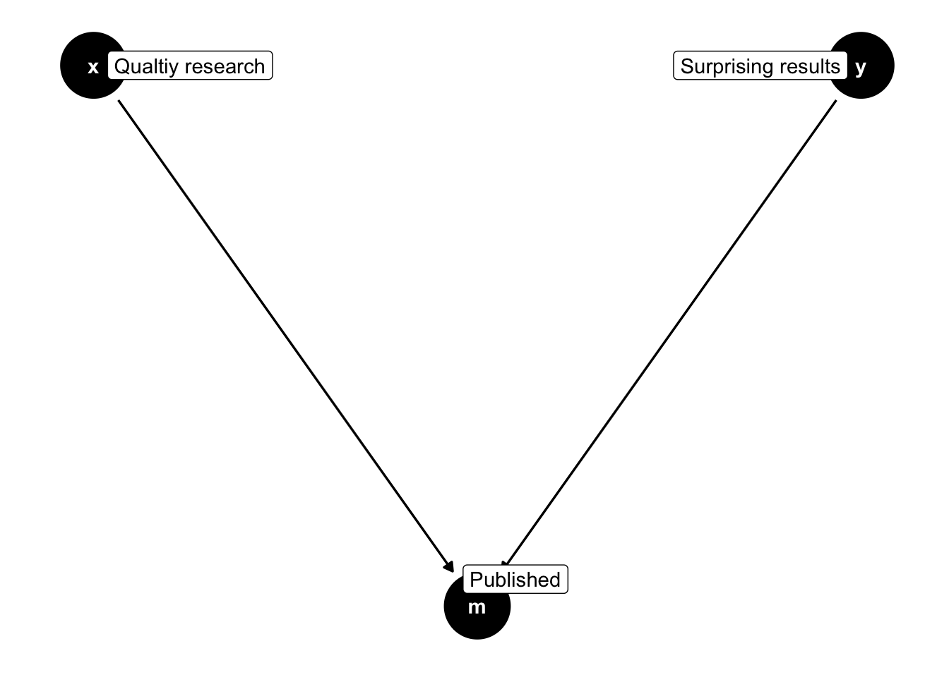
If we control for M here we are creating a backdoor path from X to Y. This is bad!
More complicated DAGs
dag = dagify(Y ~ X + P + A + I,
             X ~ P,
             exposure = "X",
             outcome = "Y")

ggdag(dag) +
  theme_dag_blank()
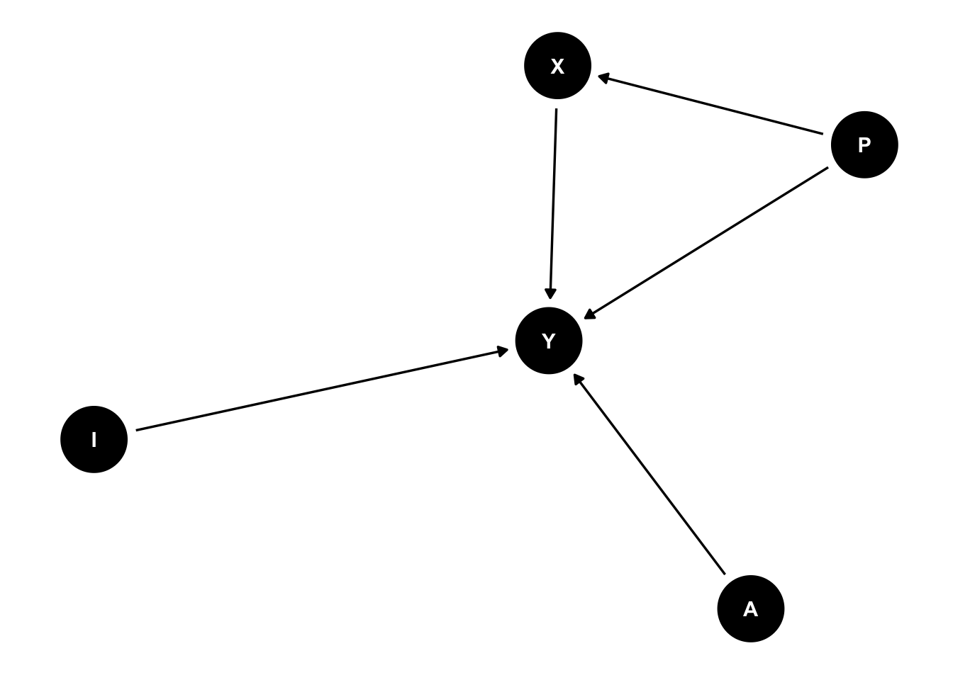
Here, we need to control for P since it is a backdoor from X to Y. Note that there are other variables that also cause Y (I and A) but we don’t need to control for them to estimate the effect of X on Y.
dag = dagify(support ~ anxiety + event,
             anxiety ~ event,
             labels = c("support" = "Support for torture",
                        "anxiety" = "Level of anxiety",
                        "event" = "Terrorism event")
)
ggdag(dag, text = FALSE, use_labels = "label") + theme_dag_blank()
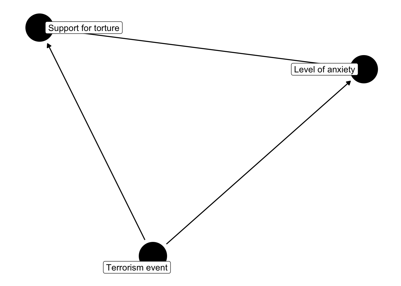
In this example from class, we want to know the effect of experiencing terrorism on support for torture. Notice the effect of terrorism on support for torture is both direct and indirect (via heightened anxiety). This is an example of a pipe; if we control for anxiety here, we are effectively controlling away part of the effect of terrorism on support for torture.
smoking_ca_dag = dagify(cardiacarrest ~ cholesterol,
                         cholesterol ~ smoking + weight,
                         smoking ~ unhealthy,
                         weight ~ unhealthy,
                         labels = c("cardiacarrest" = "Cardiac\n Arrest",
                                    "smoking" = "Drugs",
                                    "cholesterol" = "Cholesterol",
                                    "unhealthy" = "Unhealthy\n Lifestyle",
                                    "weight" = "Weight"),
                         latent = "unhealthy",
                         exposure = "smoking",
                         outcome = "cardiacarrest")

ggdag(smoking_ca_dag, text = FALSE, use_labels = "label") + theme_dag_blank()
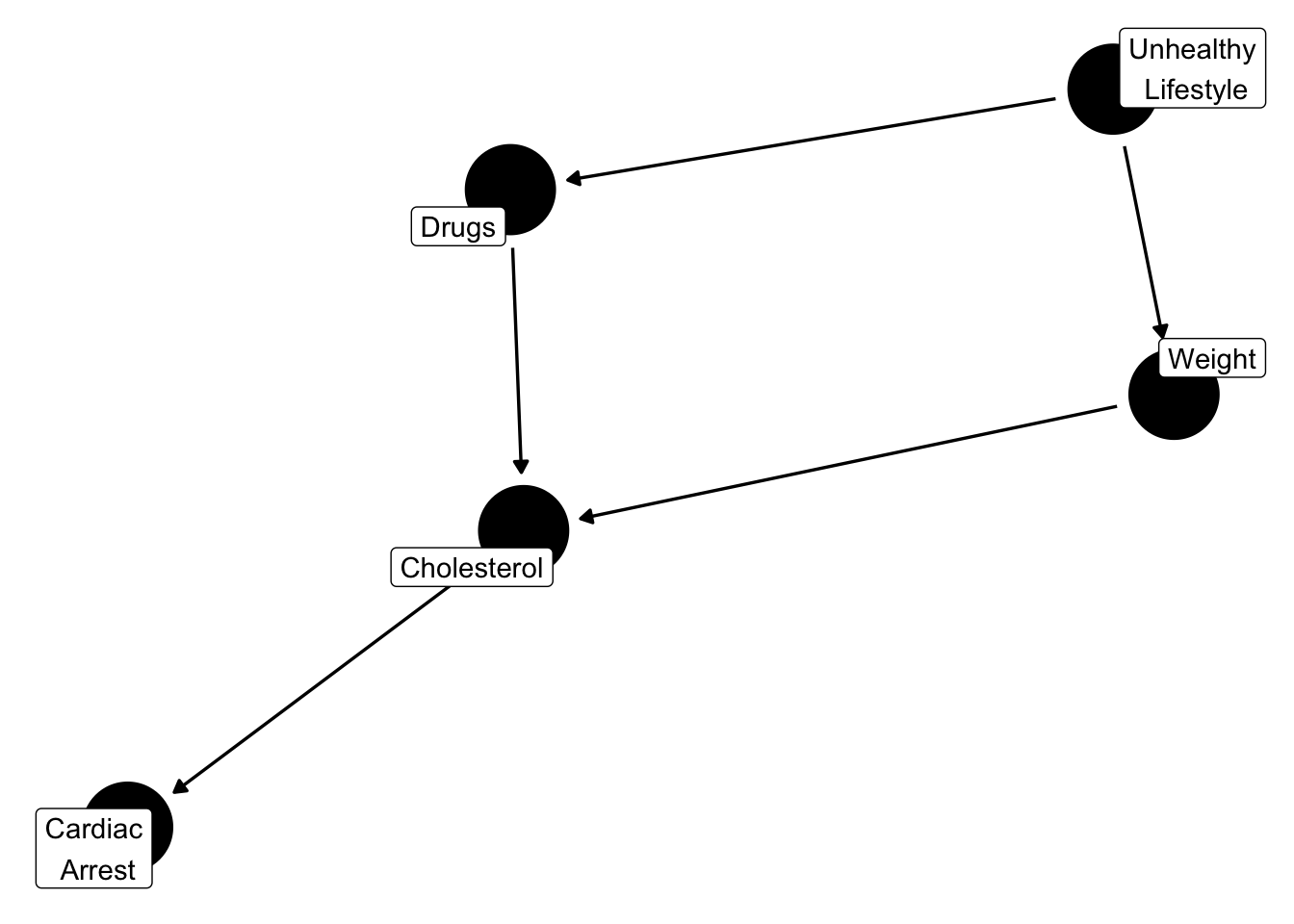
In this example we want to know the effect of drug use on cardiac arrest. Notice there is a backdoor path through unhealthy life styles, to weight, to cholesterol, and onto cardiac arrest. We want to close that backdoor path: we can control for unhealthy lifestyle, OR weight (notice how both break the chain!).
But there is also a pipe here! If we were to accidentally control for cholesterol we would be closing a front-door path (bad). So we need to avoid doing that.
dag = dagify(y ~ x + c,
       x ~ u,
       u ~ a,
       c ~ a,
       b ~ u + c,
       exposure = "x",
       outcome = "y")
ggdag(dag) + theme_dag_blank()
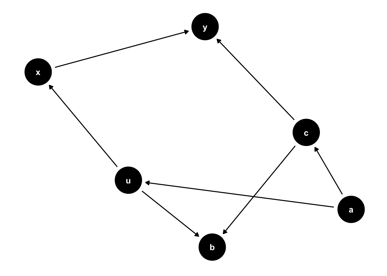
Notice the backdoor path: X <- U -> A -> C -> Y. To close it and break the chain we can control for U, A, or C.