Data Wrangling
In-class example
Here’s the code we’ll be using in class. Download it and store it with the rest of your materials for this course. If simply clicking doesn’t trigger download, you should right-click and select “save link as…”
Filtering
Often, we have a big dataset that covers lots of stuff (say, all flights coming out of NYC in 2013) but we’re only interested in a subset of those things (say, flights that arrived late over that time period). The filter() function is a way to subset operations that match some rule or set of rules (e.g., rule = “flights that arrived late”). We define these rules using
logical operators.
Examples
Let’s load the libraries.
# libraries
library(tidyverse)
library(nycflights13)
Remember you can look at the data like this.
# look at the data
View(flights) # open data in viewer
?flights # read data documentation
Let’s look at flights from February.
# look at fights, but only from February
flights %>%
  filter(month == 2)
## # A tibble: 24,951 × 19
##     year month   day dep_time sched_dep_time dep_delay arr_time sched_arr_time
##    <int> <int> <int>    <int>          <int>     <dbl>    <int>          <int>
##  1  2013     2     1      456            500        -4      652            648
##  2  2013     2     1      520            525        -5      816            820
##  3  2013     2     1      527            530        -3      837            829
##  4  2013     2     1      532            540        -8     1007           1017
##  5  2013     2     1      540            540         0      859            850
##  6  2013     2     1      552            600        -8      714            715
##  7  2013     2     1      552            600        -8      919            910
##  8  2013     2     1      552            600        -8      655            709
##  9  2013     2     1      553            600        -7      833            815
## 10  2013     2     1      553            600        -7      821            825
## # ℹ 24,941 more rows
## # ℹ 11 more variables: arr_delay <dbl>, carrier <chr>, flight <int>,
## #   tailnum <chr>, origin <chr>, dest <chr>, air_time <dbl>, distance <dbl>,
## #   hour <dbl>, minute <dbl>, time_hour <dttm>
Let’s look at flights on Valentine’s Day.
# now let's look at flights on Valentine's Day
flights %>%
  filter(month == 2) %>%
  filter(day == 14)
## # A tibble: 956 × 19
##     year month   day dep_time sched_dep_time dep_delay arr_time sched_arr_time
##    <int> <int> <int>    <int>          <int>     <dbl>    <int>          <int>
##  1  2013     2    14        7           2352        15      448            437
##  2  2013     2    14       59           2339        80      205            106
##  3  2013     2    14      454            500        -6      641            648
##  4  2013     2    14      510            515        -5      750            814
##  5  2013     2    14      531            530         1      828            831
##  6  2013     2    14      541            540         1      850            850
##  7  2013     2    14      542            545        -3     1014           1023
##  8  2013     2    14      551            600        -9      831            906
##  9  2013     2    14      552            600        -8      657            708
## 10  2013     2    14      553            600        -7      902            856
## # ℹ 946 more rows
## # ℹ 11 more variables: arr_delay <dbl>, carrier <chr>, flight <int>,
## #   tailnum <chr>, origin <chr>, dest <chr>, air_time <dbl>, distance <dbl>,
## #   hour <dbl>, minute <dbl>, time_hour <dttm>
Let’s try the OR logical operator by looking at flights going to ATL or SFO.
# try one using text and the OR symbol
# look at fights going to ATL or SFO
flights %>%
  filter(dest == "ATL" | dest == "SFO")
## # A tibble: 30,546 × 19
##     year month   day dep_time sched_dep_time dep_delay arr_time sched_arr_time
##    <int> <int> <int>    <int>          <int>     <dbl>    <int>          <int>
##  1  2013     1     1      554            600        -6      812            837
##  2  2013     1     1      558            600        -2      923            937
##  3  2013     1     1      600            600         0      837            825
##  4  2013     1     1      606            610        -4      837            845
##  5  2013     1     1      611            600        11      945            931
##  6  2013     1     1      615            615         0      833            842
##  7  2013     1     1      655            700        -5     1037           1045
##  8  2013     1     1      658            700        -2      944            939
##  9  2013     1     1      729            730        -1     1049           1115
## 10  2013     1     1      734            737        -3     1047           1113
## # ℹ 30,536 more rows
## # ℹ 11 more variables: arr_delay <dbl>, carrier <chr>, flight <int>,
## #   tailnum <chr>, origin <chr>, dest <chr>, air_time <dbl>, distance <dbl>,
## #   hour <dbl>, minute <dbl>, time_hour <dttm>
Let’s look at flights between noon and 5pm.
# try one using greater than or less than
# look at flights departing between 12pm and 5pm
flights %>%
  filter(dep_time >= 1200) %>%
  filter(dep_time <= 1700)
## # A tibble: 99,136 × 19
##     year month   day dep_time sched_dep_time dep_delay arr_time sched_arr_time
##    <int> <int> <int>    <int>          <int>     <dbl>    <int>          <int>
##  1  2013     1     1     1200           1200         0     1408           1356
##  2  2013     1     1     1202           1207        -5     1318           1314
##  3  2013     1     1     1202           1159         3     1645           1653
##  4  2013     1     1     1203           1205        -2     1501           1437
##  5  2013     1     1     1203           1200         3     1519           1545
##  6  2013     1     1     1204           1200         4     1500           1448
##  7  2013     1     1     1205           1200         5     1503           1505
##  8  2013     1     1     1206           1209        -3     1325           1328
##  9  2013     1     1     1208           1158        10     1540           1502
## 10  2013     1     1     1211           1215        -4     1423           1413
## # ℹ 99,126 more rows
## # ℹ 11 more variables: arr_delay <dbl>, carrier <chr>, flight <int>,
## #   tailnum <chr>, origin <chr>, dest <chr>, air_time <dbl>, distance <dbl>,
## #   hour <dbl>, minute <dbl>, time_hour <dttm>
Let’s look at how many flights arrived late on christmas day.
## how many flights arrived LATE, on christmas day?
late_xmas = flights %>%
  filter(arr_time > sched_arr_time) %>%
  filter(month == 12, day == 25)
Leaders
library(juanr)
leader
## # A tibble: 17,686 × 16
##    country gwcode leader gender  year yr_office   age edu     mil_service combat
##    <chr>    <dbl> <chr>  <chr>  <dbl>     <dbl> <dbl> <fct>         <dbl>  <dbl>
##  1 USA          2 Grant  M       1869         1    47 Univer…           1      1
##  2 USA          2 Grant  M       1870         2    48 Univer…           1      1
##  3 USA          2 Grant  M       1871         3    49 Univer…           1      1
##  4 USA          2 Grant  M       1872         4    50 Univer…           1      1
##  5 USA          2 Grant  M       1873         5    51 Univer…           1      1
##  6 USA          2 Grant  M       1874         6    52 Univer…           1      1
##  7 USA          2 Grant  M       1875         7    53 Univer…           1      1
##  8 USA          2 Grant  M       1876         8    54 Univer…           1      1
##  9 USA          2 Grant  M       1877         9    55 Univer…           1      1
## 10 USA          2 Hayes  M       1877         1    55 Gradua…           1      1
## # ℹ 17,676 more rows
## # ℹ 6 more variables: rebel <dbl>, yrs_exp <dbl>, phys_health <dbl>,
## #   mental_health <dbl>, will_force <dbl>, will_force_sd <dbl>
- A Vietnamese Emperor who, in his first year in office, was 11 years old. Famously depraved.
leader %>%
  # first year in office
  filter(yr_office == 1) %>%
  # age at that point
  filter(age == 11) %>%
  # vietnamese
  filter(country == "VNM")
## # A tibble: 1 × 16
##   country gwcode leader    gender  year yr_office   age edu   mil_service combat
##   <chr>    <dbl> <chr>     <chr>  <dbl>     <dbl> <dbl> <fct>       <dbl>  <dbl>
## 1 VNM        815 Thanh Th… M       1889         1    11 Seco…           0      0
## # ℹ 6 more variables: rebel <dbl>, yrs_exp <dbl>, phys_health <dbl>,
## #   mental_health <dbl>, will_force <dbl>, will_force_sd <dbl>
- Leaders with graduate degrees who in 2015 reached their 16th year in power.
leader %>%
  filter(edu == "Graduate", yr_office == 16, year == 2015)
## # A tibble: 2 × 16
##   country gwcode leader    gender  year yr_office   age edu   mil_service combat
##   <chr>    <dbl> <chr>     <chr>  <dbl>     <dbl> <dbl> <fct>       <dbl>  <dbl>
## 1 RUS        365 Putin     M       2015        16    63 Grad…           0      0
## 2 SYR        652 Bashar a… M       2015        16    50 Grad…           1      0
## # ℹ 6 more variables: rebel <dbl>, yrs_exp <dbl>, phys_health <dbl>,
## #   mental_health <dbl>, will_force <dbl>, will_force_sd <dbl>
- The number of world leaders in the post-2000 period who have known physical or mental health issues.
leader %>%
  filter((year > 2000) & (phys_health == 1 | mental_health == 1))
## # A tibble: 103 × 16
##    country gwcode leader   gender  year yr_office   age edu   mil_service combat
##    <chr>    <dbl> <chr>    <chr>  <dbl>     <dbl> <dbl> <fct>       <dbl>  <dbl>
##  1 CAN         20 Chretien M       2001         9    62 Univ…           0      0
##  2 CAN         20 Chretien M       2002        10    63 Univ…           0      0
##  3 CAN         20 Chretien M       2003        11    64 Univ…           0      0
##  4 SLV        349 Drnovsek M       2001         2    51 Grad…           0      0
##  5 SLV        349 Drnovsek M       2002         3    52 Grad…           0      0
##  6 BLR        370 Lukashe… M       2001         8    47 Grad…           1      0
##  7 BLR        370 Lukashe… M       2002         9    48 Grad…           1      0
##  8 BLR        370 Lukashe… M       2003        10    49 Grad…           1      0
##  9 BLR        370 Lukashe… M       2004        11    50 Grad…           1      0
## 10 BLR        370 Lukashe… M       2005        12    51 Grad…           1      0
## # ℹ 93 more rows
## # ℹ 6 more variables: rebel <dbl>, yrs_exp <dbl>, phys_health <dbl>,
## #   mental_health <dbl>, will_force <dbl>, will_force_sd <dbl>
Mutating
Sometimes we want to create new variables. For example, we might want to combine or alter existing variables in our dataset. The mutate() function is one way of doing this.
Let’s convert arrival delay from minutes to hours.
## convert arrival_delay to hours
new_flights = flights %>%
  mutate(arr_delay_hrs = arr_delay/60)
If you look in the dataset you will see a new variable called arr_delay_hrs.
Let’s convert distance traveled from miles to thousands of miles.
## convert distance to thousands of miles
new_flights2 = flights %>%
  mutate(dist_miles = distance/1000)
Creating categorical variables
Sometimes we want to create more complicated variables. Here’s where case_when comes into play.
Let’s create a variable that tells us what season a flight took off in.
## create a new variable called season
## that tells me if flight departed
## in summer, winter, fall, or spring
new_flights = flights %>%
  mutate(seasons = case_when(month == 6 ~ "Summer",
                             month == 7 ~ "Summer",
                             month == 8 ~ "Summer",
                             month == 9 ~ "Fall",
                             month == 10 ~ "Fall",
                             month == 11 ~ "Fall",
                             month == 12 ~ "Winter",
                             month == 1 ~ "Winter",
                             month == 2 ~ "Winter",
                             month == 3 ~ "Spring",
                             month == 4 ~ "Spring",
                             month == 5 ~ "Spring"))
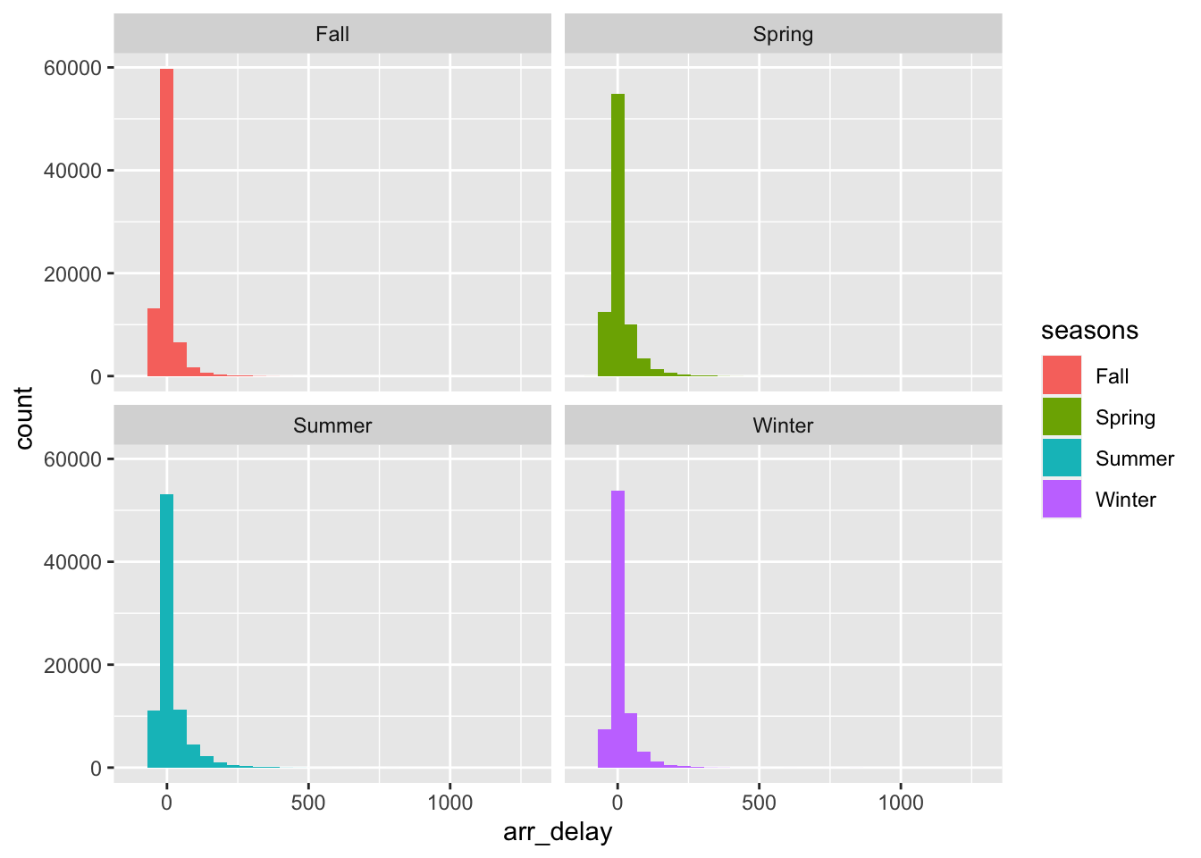
We can then plot the distribution of arrival delays by season, below.
# plot histogram of arrival delay
# separate it by season
ggplot(new_flights, aes(x = arr_delay, fill = seasons)) +
  geom_histogram() +
  facet_wrap(vars(seasons))
## `stat_bin()` using `bins = 30`. Pick better value with `binwidth`.

## Warning: Removed 9430 rows containing non-finite values (`stat_bin()`).
Let’s say we wanted to categorize flights by how late they are. See an example, below.
new_flights = flights %>%
  mutate(time_flight = case_when(arr_delay >= 120 ~ "very late",
                                 arr_delay > 0 & arr_delay < 120 ~ "a little late",
                                 arr_delay == 0 ~ "on time",
                                 arr_delay < 0 & arr_delay > -120 ~ "a little early",
                                 arr_delay <=-120 ~ "very early"))