Probability II: Bayesian Updating (answer)
The source .qmd code can be found here
The Setup
A professor wants to know whether students like his class, but he does not have a good sense of the answer beforehand (a weak prior). To learn more, he surveys students who have taken his class before.
Suppose 50 individuals are randomly chosen from the large population of students who have taken the class. Each is asked a single question with two possible responses:
- “Yes, I liked it.”
- “No, I hated it.”
Let \(\theta\) denote the proportion of the population who would answer “Yes.” The professor’s prior distribution for \(\theta\) is
$$\theta \sim \text{Beta}(1.5,\ 1.5),$$
with known parameters. In the sample, 37 students responded “Yes” and 13 responded “No.”
Big question: What can we infer about
\(\theta\)after observing the data?
This is going to be your basic setup:
# Parameters from the problem
a <- 1.5; b <- 1.5     # prior: Beta(1.5, 1.5)
n.yes <- 37; n.no <- 13 # data: 37 Yes, 13 No

# Posterior parameters
a.post <- a + n.yes
b.post <- b + n.no
1. Prior mean and standard deviation
Find the prior mean and prior standard deviation of \(\theta\).
Answer: Because I am already told that the prior is \(\theta \sim \text{Beta}(1.5,\ 1.5)\), the two parameters of the Beta distribution are \(a = b = 1.5\). Now I can just follow the formulae I was given to calculate \(E(\theta)\) and \(\text{Var}(\theta)\):
$$E(\theta) = \frac{a}{a+b} = \frac{1.5}{3} = 0.5,$$
$$\text{Var}(\theta) = \frac{ab}{(a+b)^2\,(a+b+1)} = \frac{1.5 \times 1.5}{3^2 \times 4} = \frac{2.25}{36} = \frac{1}{16},$$
so the prior standard deviation is \(\text{SD}(\theta) = \sqrt{1/16} = 0.25\).
You can also ask R to do the calculation for you, and you will get the same result:
prior.mean <- a / (a + b)
prior.var  <- (a * b) / ((a + b)^2 * (a + b + 1))
prior.sd   <- sqrt(prior.var)

c(mean = prior.mean, var = prior.var, sd = prior.sd)
##   mean    var     sd
## 0.5000 0.0625 0.2500
2. A prior probability
Find the prior probability that \(\theta < 0.6\).
Answer:
Because you already know that \(a = b = 1.5\), you can just calculate the prior probability in the Beta distribution by running the following R code:
pbeta(0.6, a, b)
## [1] 0.62647
So \(\Pr(\theta < 0.6) \approx 0.626\) under the prior.
3. The likelihood
Find the likelihood \(f(x \mid \theta)\).
Answer: Each response is a Bernoulli draw with success probability \(\theta\). With 37 “Yes” and 13 “No” responses, multiplying the 50 Bernoulli probabilities together gives our likelihood (the same form as a binomial):
$$f(x \mid \theta) \propto \theta^{37}\,(1-\theta)^{13}.$$
4. The posterior distribution
Find the posterior distribution \(\xi(\theta \mid x)\).
Answer: Because we have already known the likelihood distribution from the above, and we also know the prior distribution from the hint, now we can just multiply the likelihood by the prior:
$$\begin{aligned} \xi(\theta \mid x) &\propto f(x \mid \theta) \times \xi(\theta) \\ &\propto \theta^{37}(1-\theta)^{13} \times \theta^{1.5-1}(1-\theta)^{1.5-1} \\ &= \theta^{38.5-1}(1-\theta)^{14.5-1}. \end{aligned}$$
The right-hand side is the kernel of a Beta distribution (meaning that the posterior is again a Beta distribution, just like the prior), so the posterior is
$$\theta \mid x \sim \text{Beta}(38.5,\ 14.5).$$
where \(a = 38.5\) and \(b = 14.5\) are our new parameters for the posterior Beta distribution.
This confirms a general result in Bayesian statistics (the Beta prior is conjugate to the binomial likelihood): a \(\text{Beta}(a, b)\) prior combined with \(n_{\text{yes}}\) successes and \(n_{\text{no}}\) failures gives a \(\text{Beta}(a + n_{\text{yes}},\ b + n_{\text{no}})\) posterior.
5. Plot the prior and posterior
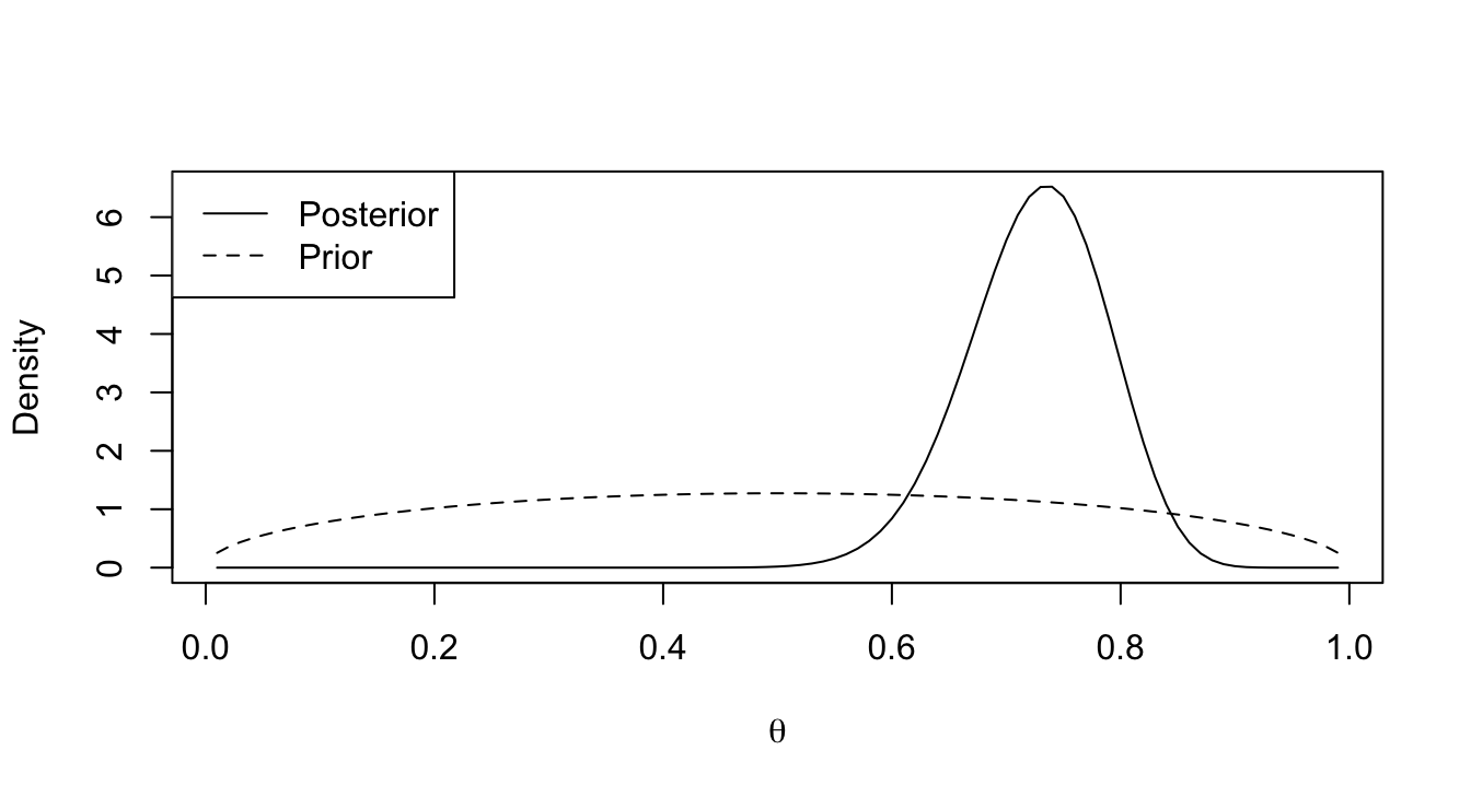
Okay great! We have derived the posterior distribution from the multiplication between our likelihood and the prior. Now we can ask R to plot the Bayesian parameter \(\theta\) updating for us.
Note: We plot the prior density \(\xi(\theta)\) and the posterior density \(\xi(\theta \mid x)\) on the same axes for the ease of comparison between the prior \(\theta\) and posterior \(\theta\).
Answer:
theta     <- seq(0.01, 0.99, 0.01)         # theta is a probability which lies
# in between (0, 1), so generate many of them between 0 and 1 in a sequence
prior     <- dbeta(theta, a, b)             # Beta(a =1.5, b=1.5)
posterior <- dbeta(theta, a.post, b.post)   # Beta(a=38.5, b=14.5)

plot(theta, posterior, type = "l",
     xlab = expression(theta), ylab = "Density")
lines(theta, prior, lty = 2)
legend("topleft", legend = c("Posterior", "Prior"), lty = c(1, 2))
6. Interpretation
Explain what you have learned by generating the plot. How did the data change the professor’s beliefs about \(\theta\)?
Answer: The plot shows how the data update the professor’s belief about \(\theta\), the proportion of students who would say “Yes.”
- The prior,
\(\text{Beta}(1.5, 1.5)\), is nearly flat and centered at 0.5. The professor started without a strong guess about\(\theta\). - After observing 37 “Yes” and 13 “No,” the posterior,
\(\text{Beta}(38.5, 14.5)\), is much more concentrated and has shifted to the right. - You can also get the exact mean and variance by calculating them by hand:
Following the above-mentioned formulas for the Beta distribution:
$$E(\theta) = \frac{a}{a+b}$$
$$\text{Var}(\theta) = \frac{ab}{(a+b)^2\,(a+b+1)}$$
I am being too lazy, so I will just ask R to do the hand calculation for me:
# Parameters from the problem
# a <- 1.5; b <- 1.5     # prior: Beta(1.5, 1.5)
# n.yes <- 37; n.no <- 13 # data: 37 Yes, 13 No

# # Posterior parameters
# a.post <- a + n.yes
# b.post <- b + n.no

post.mean <- a.post / (a.post + b.post)
post.sd   <- sqrt((a.post * b.post) /
                 ((a.post + b.post)^2 * (a.post + b.post + 1)))

c(mean = post.mean, sd = post.sd)
##       mean         sd
## 0.72641509 0.06066548
# Posterior Pr(theta < 0.6); compare with the prior answer in Q2
pbeta(0.6, a.post, b.post)
## [1] 0.02490528
The posterior mean is about 0.73 and the posterior standard deviation shrinks from 0.25 to about 0.06.
Now if we want to know the probability that \(\theta\) falls under the threshold of 0.6 (i.e., \(\Pr(\theta < 0.6)\)), the answer tells us that it falls from about 0.63 under the prior to about 0.025 under the posterior.
Because the prior was weak, the data dominate: the professor now believes fairly firmly that most students (roughly 73%) liked the class.