The goal of the day

• Show you that some tricky math problems can be solved by modern computing power
• We use a very classical math problem as an example

The Birthday Problem

There are 5 people in a room. Assume each person’s birthday is equally likely to be any of the 365 days of the year (no leap babies) and birthdays are independent. What is the probability that at least one pair of people have the same birthday (at least one match)?

1. Let’s do it mathmetically

1 – Probability of no match = Probability of at least one match

For the first person, there are no birthdays already covered, which means that there is a 365/365 chance that there is not a shared birthday. That makes sense. We have just one person.

\(1 - (\frac{365}{365}) = 0\)

Now, let’s add in the second person to test the match. The first person covers one possible birthday, so the second person has a 364/365 chance of not sharing the same day. We need to multiply the probabilities of the first two people and subtract from one.

\(1 - (\frac{365}{365}) \times (\frac{364}{365}) = 0.0027\)

For the third person, the previous two people cover two dates. Hence, the third person has a probability of 363/365 for not sharing a birthday.

\(1 - (\frac{365}{365}) \times (\frac{364}{365}) \times (\frac{363}{365}) = 0.0082\)

Now, you’re seeing the pattern for how to calculate the probability for a given number of people. For a 5 person room, the probability of finding at least one match is:

\(1 - (\frac{365}{365}) \times (\frac{364}{365}) \times (\frac{363}{365}) \times (\frac{362}{365}) \times (\frac{361}{365}) = 0.027\)

2. Let’s do it in R by simulation

Let’s do a first 10k random draw, and see what happens?

set.seed(1)
n <- 5
match <- 0

# Simulate a random sample of 10000 rooms and check for matches in each room
sam = 10000
# i = 1
for(i in 1:sam){
  birthdays <- sample(365, n, replace = TRUE)
  # if any of them are identical, I save the match and count 1
  if(length(unique(birthdays)) < n){
    match <- match + 1 # this is a counter
  } 
}

# Calculate the estimated probability of a match and print it
p_match <- match / sam # how many matches you found in your simulation of n
print(p_match)

## [1] 0.0288

It turns out to be 0.0288, which is quite similar to our math result of 0.027

Let’s do a second 10k random draw. To be able to do this, we just change the seed number from set.seed(1) to set.seed(123).

set.seed(123)
n <- 5
match <- 0

# Simulate a random sample of n rooms and check for matches in each room
sam = 10000

for(i in 1:sam){
  birthdays <- sample(365, n, replace = TRUE)
  if(length(unique(birthdays)) < n){
    match <- match + 1
  } 
}

# Calculate the estimated probability of a match and print it
p_match <- match / sam
print(p_match)

## [1] 0.0283

It turns out to be 0.0283, which is again quite similar to our math result of 0.027

We may want to increase the sample size so that we don’t have to repeat our random draws that many times to get to a conclusive probability. Let’s increase the sample size from 10k to 50k.

set.seed(1)
n <- 5
match <- 0

# Simulate a random sample of n rooms and check for matches in each room

sam = 50000

for(i in 1:sam){
  birthdays <- sample(365, n, replace = TRUE)
  if(length(unique(birthdays)) < n){
    match <- match + 1
  } 
}

# Calculate the estimated probability of a match and print it
p_match <- match / sam
print(p_match)

## [1] 0.02676

Fortunately, my computer is fast enough and gives me a result less than a second. The probability is 0.02676, which is a different but still similar to our math result.

How about we perform multiple 10k random draws and plot the distribution of the probability?

set.seed(1)

iterations = 300 # n draws
p_match_out = NULL # create an empty vector to store estimated probs.

# jj =1

# outer loop over n draws
for(jj in 1:iterations){
  
  # inner loop, per draw
  sam = 10000 # sample size for one draw
  n <- 5
  match <- 0 
  for(ii in 1:sam){
    birthdays <- sample(365, n, replace = TRUE)
    if(length(unique(birthdays)) < n){
      match <- match + 1
    } 
  }
  
  # Calculate the estimated probability of a match and print it
  p_match <- match / sam
  p_match_out <- c(p_match_out, p_match)
  rm(match, p_match)
}

p_match_out 

##   [1] 0.0288 0.0266 0.0263 0.0263 0.0258 0.0252 0.0271 0.0281 0.0272 0.0250
##  [11] 0.0254 0.0267 0.0272 0.0248 0.0273 0.0283 0.0267 0.0278 0.0275 0.0269
##  [21] 0.0284 0.0281 0.0285 0.0255 0.0248 0.0280 0.0261 0.0281 0.0266 0.0267
##  [31] 0.0282 0.0271 0.0301 0.0288 0.0272 0.0284 0.0252 0.0237 0.0281 0.0257
##  [41] 0.0256 0.0275 0.0274 0.0271 0.0251 0.0263 0.0281 0.0287 0.0284 0.0270
##  [51] 0.0263 0.0283 0.0278 0.0259 0.0286 0.0294 0.0279 0.0292 0.0263 0.0285
##  [61] 0.0276 0.0271 0.0255 0.0253 0.0253 0.0292 0.0274 0.0287 0.0255 0.0319
##  [71] 0.0262 0.0281 0.0286 0.0260 0.0282 0.0286 0.0243 0.0277 0.0287 0.0258
##  [81] 0.0255 0.0261 0.0275 0.0273 0.0291 0.0277 0.0285 0.0261 0.0264 0.0257
##  [91] 0.0280 0.0262 0.0302 0.0290 0.0271 0.0250 0.0265 0.0293 0.0256 0.0287
## [101] 0.0257 0.0235 0.0273 0.0279 0.0279 0.0244 0.0302 0.0277 0.0299 0.0294
## [111] 0.0290 0.0278 0.0281 0.0294 0.0272 0.0304 0.0294 0.0276 0.0285 0.0234
## [121] 0.0300 0.0290 0.0254 0.0305 0.0290 0.0294 0.0299 0.0248 0.0281 0.0268
## [131] 0.0291 0.0251 0.0279 0.0272 0.0264 0.0264 0.0298 0.0252 0.0247 0.0255
## [141] 0.0249 0.0265 0.0297 0.0287 0.0258 0.0277 0.0264 0.0265 0.0279 0.0263
## [151] 0.0264 0.0269 0.0277 0.0284 0.0268 0.0280 0.0262 0.0259 0.0283 0.0291
## [161] 0.0266 0.0262 0.0267 0.0251 0.0258 0.0267 0.0268 0.0288 0.0256 0.0284
## [171] 0.0267 0.0246 0.0279 0.0257 0.0314 0.0267 0.0262 0.0262 0.0291 0.0274
## [181] 0.0279 0.0274 0.0281 0.0279 0.0276 0.0279 0.0250 0.0281 0.0238 0.0278
## [191] 0.0286 0.0291 0.0256 0.0257 0.0250 0.0252 0.0278 0.0281 0.0280 0.0277
## [201] 0.0250 0.0304 0.0286 0.0271 0.0269 0.0266 0.0277 0.0281 0.0272 0.0267
## [211] 0.0280 0.0279 0.0295 0.0284 0.0287 0.0271 0.0230 0.0280 0.0312 0.0265
## [221] 0.0293 0.0288 0.0257 0.0244 0.0271 0.0251 0.0300 0.0286 0.0291 0.0257
## [231] 0.0271 0.0285 0.0263 0.0240 0.0277 0.0269 0.0256 0.0288 0.0267 0.0286
## [241] 0.0254 0.0262 0.0247 0.0273 0.0295 0.0267 0.0269 0.0268 0.0271 0.0267
## [251] 0.0278 0.0273 0.0256 0.0234 0.0269 0.0291 0.0275 0.0256 0.0262 0.0250
## [261] 0.0264 0.0277 0.0283 0.0253 0.0259 0.0291 0.0274 0.0266 0.0266 0.0290
## [271] 0.0264 0.0217 0.0254 0.0278 0.0270 0.0259 0.0240 0.0263 0.0274 0.0269
## [281] 0.0248 0.0273 0.0254 0.0248 0.0246 0.0280 0.0254 0.0278 0.0260 0.0249
## [291] 0.0267 0.0253 0.0282 0.0255 0.0245 0.0295 0.0273 0.0255 0.0236 0.0270

mean(p_match_out)

## [1] 0.027101

# Let's plot the prob distribution
hist(p_match_out, freq = FALSE, main = "Histogram and density")

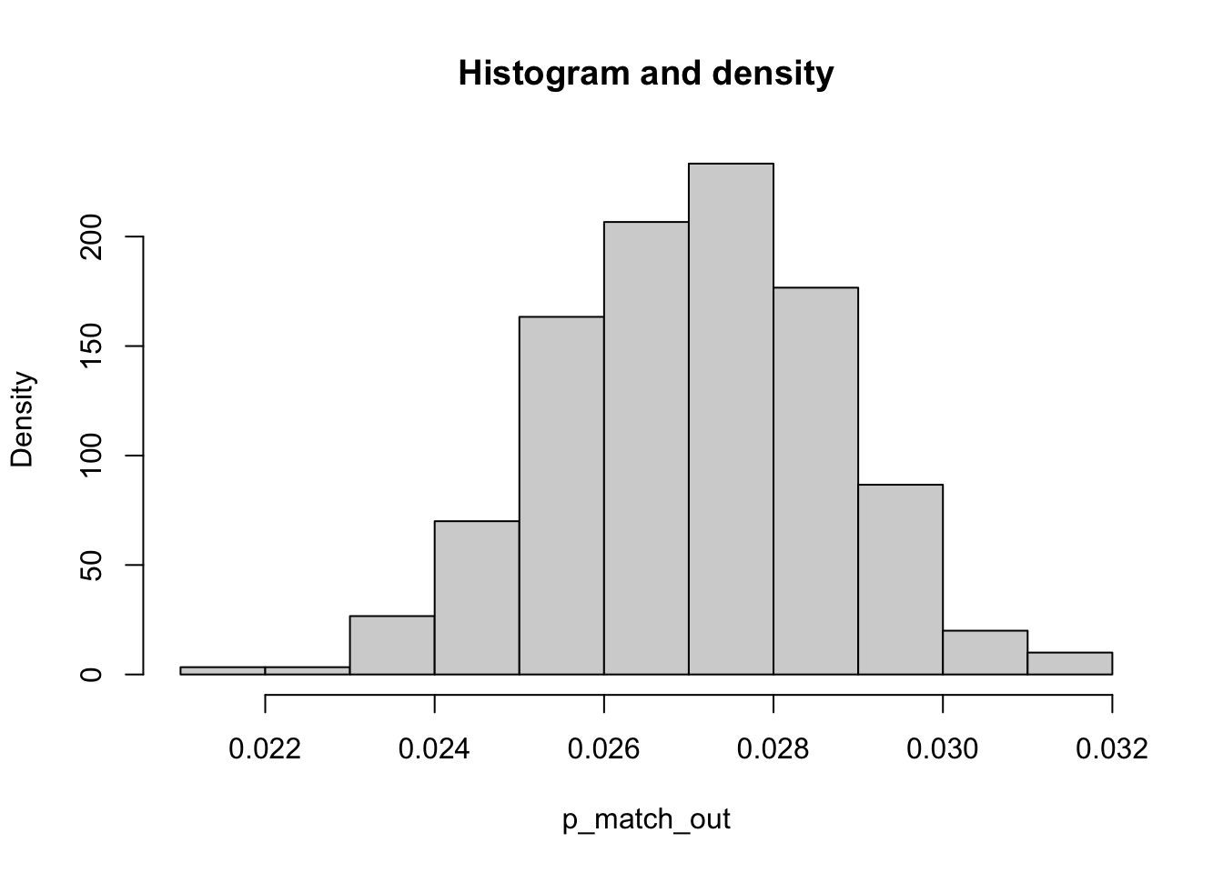
See! 0.027101 is pretty close to what we had before using a math trick. Now, you don’t need math anymore, just use the computing power on your laptop to get n numbers of random draws/simulations, and get the same result. This is the power of simulation.

Simulation: This is the heart of Bayesian statistics where you utilize the computational power to give you a good guess of the estimated probability-just repeat your random draws many times! It is more intuitive and closer to how our brain functions. With modern computational power, we can do this calculation very quickly without even needing to do any math. Just ask your computer to do thousands of simulation and then tells you the result.