Prediction
Data for this lab can be found here
# Preparation -------------------------------------------------------------
rm(list = ls())         # delete everything in the memory
library(tidyverse)
library(foreign)        # for read.dta
library(stargazer)      # Regression table
library(pscl)           # for hitmiss
library(ROCR)           # for ROC curve
library(separationplot) # separation plot
Fearon & Laitin’s (2003) data set
fl <- read.dta("/Users/howardliu/methodsPol/content/class/repdata.dta")
# For variable descriptions, see the bottom of this file.
Explore the DVs (civil war onset & ethnic war onset)
table(fl $ onset)
##
##    0    1    4
## 6499  110    1
table(fl $ ethonset)
##
##    0    1    4
## 6535   74    1
For some reason, one case is coded as 4. Let’s change the case where onset=4 to onset=1
fl $ onset[fl $ onset == 4] <- 1
fl $ ethonset[fl $ ethonset == 4] <- 1
Estimate logit models
The first three models reported in Table 1 on page 84. But we need to fit/train these models by in-sample data, so first we need to subset a training and then a test set. The idea of real prediction relies on us using old data to predict new data in our sample. So let’s hold out the last ten years in our data as our test set.
Note that all data used here are the training set, not the test set!
fl$year %>% unique
##  [1] 1945 1946 1947 1948 1949 1950 1951 1952 1953 1954 1955 1956 1957 1958 1959
## [16] 1960 1961 1962 1963 1964 1965 1966 1967 1968 1969 1970 1971 1972 1973 1974
## [31] 1975 1976 1977 1978 1979 1980 1981 1982 1983 1984 1985 1986 1987 1988 1989
## [46] 1990 1991 1992 1993 1994 1995 1996 1997 1998 1999
splityear <- 1990

# Split into training and test sets
train <- subset(fl, year < splityear)
test <- subset(fl, year >= splityear)


mod1 <- glm(onset ~
              warl + gdpenl + lpopl1 + lmtnest + ncontig +
              Oil + nwstate + instab + polity2l +
              ethfrac + relfrac,
            family = binomial(link = logit),
            data = train)

mod2 <- glm(ethonset ~
              warl + gdpenl + lpopl1 + lmtnest + ncontig +
              Oil + nwstate + instab + polity2l +
              ethfrac + relfrac,
            family = binomial(link = logit),
            data = train)

mod3 <- glm(onset ~
              warl + gdpenl + lpopl1 + lmtnest + ncontig +
              Oil + nwstate + instab +
              ethfrac + relfrac + anocl + deml,
            family = binomial(link = logit),
            data = train)
Simple stargazer table
stargazer(mod1, mod3, type = "text")
##
## ==============================================
##                       Dependent variable:
##                   ----------------------------
##                              onset
##                        (1)            (2)
## ----------------------------------------------
## warl                -1.113***      -1.100***
##                      (0.406)        (0.405)
##
## gdpenl              -0.351***      -0.335***
##                      (0.085)        (0.084)
##
## lpopl1               0.259***      0.264***
##                      (0.085)        (0.085)
##
## lmtnest              0.198**        0.187*
##                      (0.099)        (0.099)
##
## ncontig               0.425          0.424
##                      (0.320)        (0.317)
##
## Oil                  0.791**        0.738**
##                      (0.337)        (0.336)
##
## nwstate              1.482***      1.450***
##                      (0.408)        (0.409)
##
## instab                0.453          0.399
##                      (0.289)        (0.294)
##
## polity2l              0.031
##                      (0.019)
##
## ethfrac               0.176          0.191
##                      (0.429)        (0.425)
##
## relfrac               -0.075         0.022
##                      (0.592)        (0.595)
##
## anocl                               0.465*
##                                     (0.281)
##
## deml                                 0.450
##                                     (0.340)
##
## Constant            -6.460***      -6.825***
##                      (0.843)        (0.864)
##
## ----------------------------------------------
## Observations          4,943          4,943
## Log Likelihood       -366.336      -365.974
## Akaike Inf. Crit.    756.672        757.949
## ==============================================
## Note:              *p<0.1; **p<0.05; ***p<0.01
Stargazer table with options
stargazer(mod1, mod2, mod3, type = "text",
          dep.var.labels=c("Civil War","Ethnic War","Civil War"),
          covariate.labels=c("Prior war",
                             "Per capita income",
                             "log(population)",
                             "log(% mountanious)",
                             "Noncontiguous state",
                             "Oil exporter",
                             "New state",
                             "Instability",
                             "Democracy",
                             "Ethnic fractionalization",
                             "Religious fractionalization",
                             "Anocracy",
                             "Democracy")
          )
##
## ==========================================================
##                                  Dependent variable:
##                             ------------------------------
##                             Civil War Ethnic War Civil War
##                                (1)       (2)        (3)
## ----------------------------------------------------------
## Prior war                   -1.113*** -1.425***  -1.100***
##                              (0.406)   (0.528)    (0.405)
##
## Per capita income           -0.351*** -0.379***  -0.335***
##                              (0.085)   (0.112)    (0.084)
##
## log(population)             0.259***   0.426***  0.264***
##                              (0.085)   (0.103)    (0.085)
##
## log(% mountanious)           0.198**    0.152     0.187*
##                              (0.099)   (0.132)    (0.099)
##
## Noncontiguous state           0.425     0.309      0.424
##                              (0.320)   (0.401)    (0.317)
##
## Oil exporter                 0.791**   1.044**    0.738**
##                              (0.337)   (0.407)    (0.336)
##
## New state                   1.482***   1.574***  1.450***
##                              (0.408)   (0.480)    (0.409)
##
## Instability                   0.453     0.107      0.399
##                              (0.289)   (0.407)    (0.294)
##
## Democracy                     0.031     0.039
##                              (0.019)   (0.025)
##
## Ethnic fractionalization      0.176     0.976*     0.191
##                              (0.429)   (0.565)    (0.425)
##
## Religious fractionalization  -0.075     0.946      0.022
##                              (0.592)   (0.793)    (0.595)
##
## Anocracy                                          0.465*
##                                                   (0.281)
##
## Democracy                                          0.450
##                                                   (0.340)
##
## Constant                    -6.460*** -9.136***  -6.825***
##                              (0.843)   (1.120)    (0.864)
##
## ----------------------------------------------------------
## Observations                  4,943     4,943      4,943
## Log Likelihood              -366.336   -234.978  -365.974
## Akaike Inf. Crit.            756.672   493.957    757.949
## ==========================================================
## Note:                          *p<0.1; **p<0.05; ***p<0.01
See what parts of the output are changed with these two options. Note: “covariate” means “independent variable”.
1. Percentage correctly predicted
As we learned in the lecture, we use the hitmiss function included in the pscl package to obtain percentage correctly predicted (PCP).
# PCP with threshold = 0.5 (default)

hitmiss(mod1)
## Classification Threshold = 0.5
##         y=0 y=1
## yhat=0 4864  79
## yhat=1    0   0
## Percent Correctly Predicted = 98.4%
## Percent Correctly Predicted = 100%, for y = 0
## Percent Correctly Predicted = 0%  for y = 1
## Null Model Correctly Predicts 98.4%

## [1]  98.40178 100.00000   0.00000
# PCP with lower threshold

hitmiss(mod1, k = 0.4)
## Classification Threshold = 0.4
##         y=0 y=1
## yhat=0 4863  78
## yhat=1    1   1
## Percent Correctly Predicted = 98.4%
## Percent Correctly Predicted = 99.98%, for y = 0
## Percent Correctly Predicted = 1.266%  for y = 1
## Null Model Correctly Predicts 98.4%

## [1] 98.401780 99.979441  1.265823
hitmiss(mod1, k = 0.3)
## Classification Threshold = 0.3
##         y=0 y=1
## yhat=0 4863  78
## yhat=1    1   1
## Percent Correctly Predicted = 98.4%
## Percent Correctly Predicted = 99.98%, for y = 0
## Percent Correctly Predicted = 1.266%  for y = 1
## Null Model Correctly Predicts 98.4%

## [1] 98.401780 99.979441  1.265823
hitmiss(mod1, k = 0.2)
## Classification Threshold = 0.2
##         y=0 y=1
## yhat=0 4861  77
## yhat=1    3   2
## Percent Correctly Predicted = 98.38%
## Percent Correctly Predicted = 99.94%, for y = 0
## Percent Correctly Predicted = 2.532%  for y = 1
## Null Model Correctly Predicts 98.4%

## [1] 98.381550 99.938322  2.531646
hitmiss(mod1, k = 0.1)
## Classification Threshold = 0.1
##         y=0 y=1
## yhat=0 4822  68
## yhat=1   42  11
## Percent Correctly Predicted = 97.77%
## Percent Correctly Predicted = 99.14%, for y = 0
## Percent Correctly Predicted = 13.92%  for y = 1
## Null Model Correctly Predicts 98.4%

## [1] 97.77463 99.13651 13.92405
hitmiss(mod1, k = 0.05)
## Classification Threshold = 0.05
##         y=0 y=1
## yhat=0 4668  61
## yhat=1  196  18
## Percent Correctly Predicted = 94.8%
## Percent Correctly Predicted = 95.97%, for y = 0
## Percent Correctly Predicted = 22.78%  for y = 1
## Null Model Correctly Predicts 98.4%

## [1] 94.80073 95.97039 22.78481
hitmiss(mod1, k = 0)
## Classification Threshold = 0
##         y=0 y=1
## yhat=0    0   0
## yhat=1 4864  79
## Percent Correctly Predicted = 1.598%
## Percent Correctly Predicted = 0%, for y = 0
## Percent Correctly Predicted = 100%  for y = 1
## Null Model Correctly Predicts 98.4%

## [1]   1.59822   0.00000 100.00000
# PCP with greater threshold

hitmiss(mod1, k = 0.4)
## Classification Threshold = 0.4
##         y=0 y=1
## yhat=0 4863  78
## yhat=1    1   1
## Percent Correctly Predicted = 98.4%
## Percent Correctly Predicted = 99.98%, for y = 0
## Percent Correctly Predicted = 1.266%  for y = 1
## Null Model Correctly Predicts 98.4%

## [1] 98.401780 99.979441  1.265823
hitmiss(mod1, k = 0.5)
## Classification Threshold = 0.5
##         y=0 y=1
## yhat=0 4864  79
## yhat=1    0   0
## Percent Correctly Predicted = 98.4%
## Percent Correctly Predicted = 100%, for y = 0
## Percent Correctly Predicted = 0%  for y = 1
## Null Model Correctly Predicts 98.4%

## [1]  98.40178 100.00000   0.00000
hitmiss(mod1, k = 0.6)
## Classification Threshold = 0.6
##         y=0 y=1
## yhat=0 4864  79
## yhat=1    0   0
## Percent Correctly Predicted = 98.4%
## Percent Correctly Predicted = 100%, for y = 0
## Percent Correctly Predicted = 0%  for y = 1
## Null Model Correctly Predicts 98.4%

## [1]  98.40178 100.00000   0.00000
hitmiss(mod1, k = 0.8)
## Classification Threshold = 0.8
##         y=0 y=1
## yhat=0 4864  79
## yhat=1    0   0
## Percent Correctly Predicted = 98.4%
## Percent Correctly Predicted = 100%, for y = 0
## Percent Correctly Predicted = 0%  for y = 1
## Null Model Correctly Predicts 98.4%

## [1]  98.40178 100.00000   0.00000
hitmiss(mod1, k = 1)
## Classification Threshold = 1
##         y=0 y=1
## yhat=0 4864  79
## yhat=1    0   0
## Percent Correctly Predicted = 98.4%
## Percent Correctly Predicted = 100%, for y = 0
## Percent Correctly Predicted = 0%  for y = 1
## Null Model Correctly Predicts 98.4%

## [1]  98.40178 100.00000   0.00000
As I mentioned, PCP is sensitive to threshold and so we don’t usually rely on PCP.
ROC Curve
We use the ROCR package to draw ROC curves. ROCR produces a ROC curve in three steps.
-
We first need to obtain predicted probabilities for each observation. This is done with the predict command (training set).
-
We then combine the predicted probabilities with actual outcomes (0s and 1s). This is done with the prediction command.
-
We produce true positive rate and false positive rate to be plotted. This is done with the performance command (test set).
Step 1
Obtain predicted probabilities, and store them in an object.
# We do this for mod1
pred.fl1 <- predict(mod1, newdata = test, type = "response") ## This is crucial, don't forget to use newdata!!

# The predict function calculates the predicted values (such as Y-hat or P-hat)
# based on a fitted regression object. By default, it calculates Y-hat.
# Recall that, with logit models, y-hat (y_star-hat) is not something we are
# interested in. We are interested in P-hat = lambda(y_star-hat).
# To obtain P-hat, we use the type = "response" option.

head(pred.fl1)
##           46           47           48           49           50           51
## 0.0002737127 0.0002782963 0.0003278214 0.0002905196 0.0002661136 0.0002238588
Step 2
We combine the predicted values with actual outcome. The actual outcomes are onset from the fl data set. Note that the function we use here is prediction, not predict.
# prediction.fl1 <- prediction(pred.fl1, test$onset )

# We got an error message!
# This happened because pred.fl1 and fl $ onset are of different lengths.

length(na.omit(pred.fl1))
## [1] 1384
length(na.omit(test $ onset))
## [1] 1534
# pred.fl1 is shorter than fl $ onset because of missing values.
# Let's delete observations with missing values using the na.omit function.

eval <- data.frame(cbind(pred.fl1, test $ onset)); eval <- na.omit(eval)
colnames(eval) <- c("pred.fl1", "onset")
Re-do the second step
prediction.fl1 <- prediction(eval$pred.fl1, eval$ onset)
Step 3
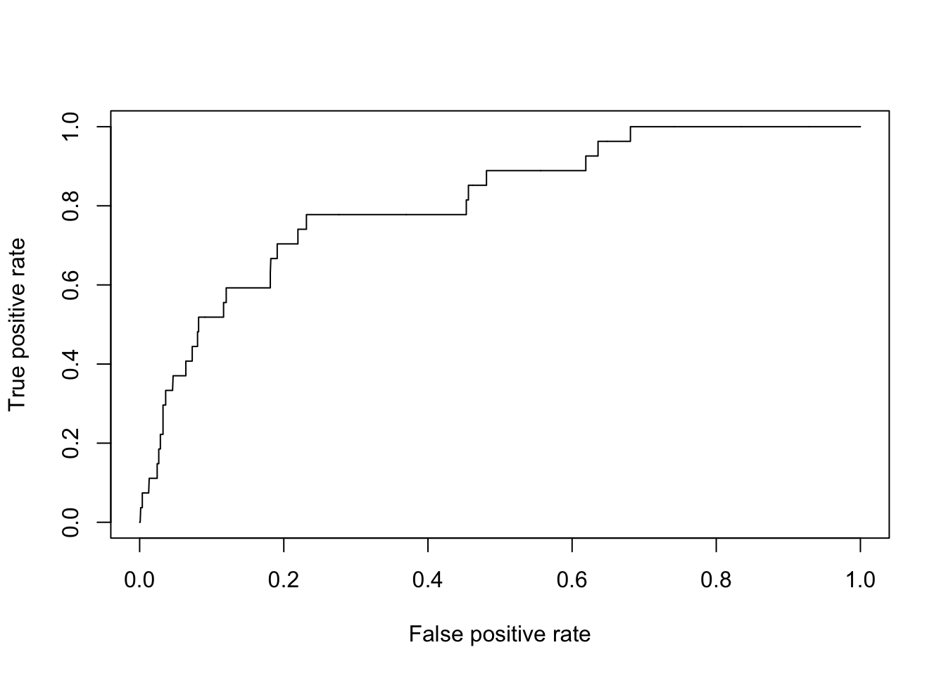
Finally, we produce what’s to be plotted using the performance function. tpr and fpr mean true positive rate and false positive rate, respectively. These are plotted in a ROC curve.
perf.fl1 <- performance(prediction.fl1, "tpr", "fpr")
Then, we can plot it
plot(perf.fl1)
To summarize, we only need a few lines of code:
pred.fl1 <- predict(mod1, newdata = test, type = "response")  # predict
eval <- data.frame(cbind(pred.fl1, test $ onset)); eval <- na.omit(eval)  # evaluation table
colnames(eval) <- c("pred.fl1", "onset")
prediction.fl1 <- prediction(eval$pred.fl1, eval$onset) # prediction
perf.fl1 <- performance(prediction.fl1, "tpr", "fpr")  # performance
plot(perf.fl1)                                         # plot

We usually draw a 45-degree line for baseline. To add a line y = a + b * x, we use the abline function.
{plot(perf.fl1)                                         # plot
abline(a = 0, b = 1, lty = "dashed", col = "gray")}
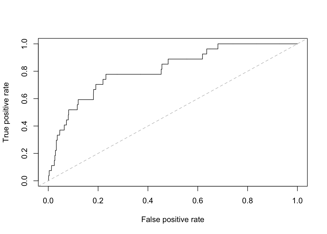 Notice that “a = 0, b = 1” means we are plotting y = 0 + 1 \* x, or y = x, which is a 45-degree line.
The lty option specifies line type (Line TYpe), which could be “solid”, “dashed”, “dotted”, etc., or 1, 2, 3,… The col option specifies the color.
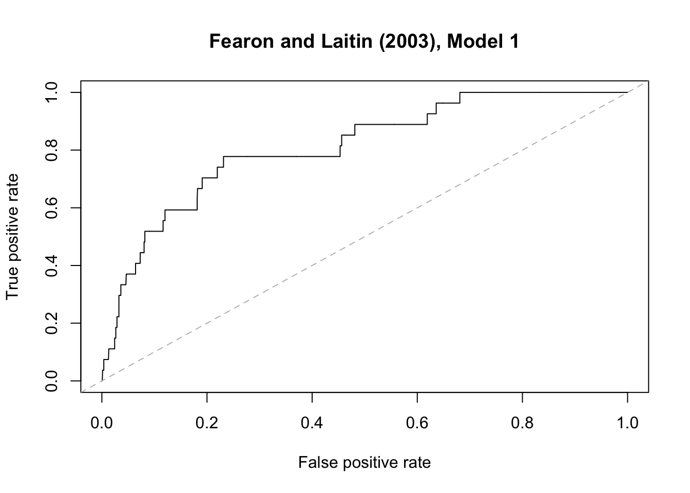
To export the graph into a PDF file:
# pdf("roc1.pdf")
{plot(perf.fl1, main = "Fearon and Laitin (2003), Model 1")
abline(a = 0, b = 1, lty = "dashed", col="gray")}
# dev.off()
Let’s do this with other models, and combine the plot
Model 3
pred.fl3 <- predict(mod3, newdata = test, type = "response")
eval <- data.frame(cbind(pred.fl3, test $ onset)); eval <- na.omit(eval)
colnames(eval) <- c("pred.fl3", "onset")
prediction.fl3 <- prediction(eval$pred.fl3, eval$onset)
perf.fl3 <- performance(prediction.fl3, "tpr", "fpr")


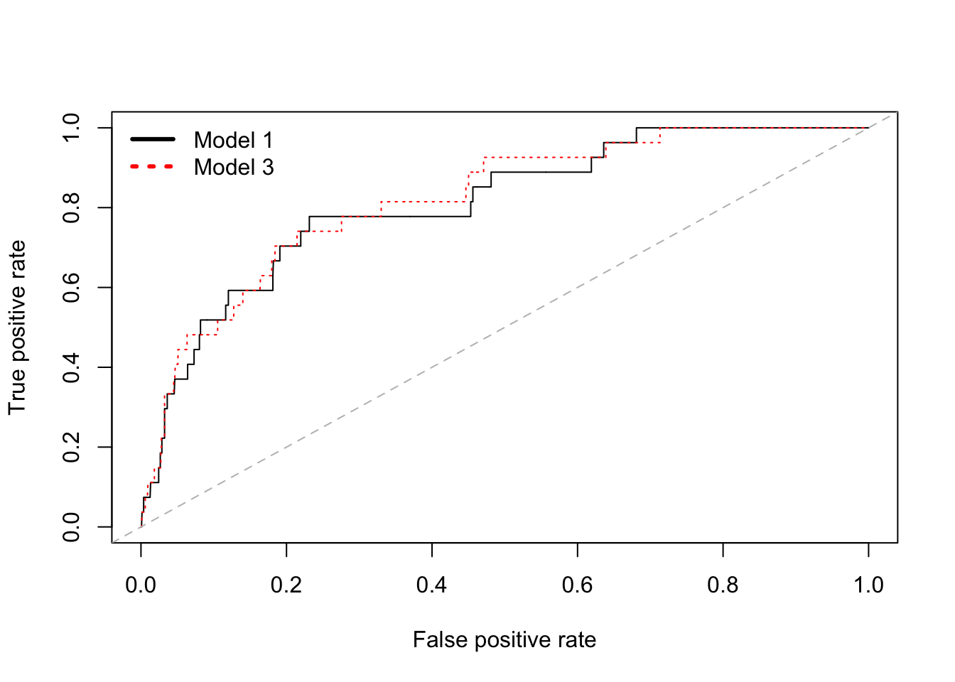
# A graph that shows ROC curves for both model 1 and model 3
# pdf("roc2.pdf")
{plot(perf.fl1)                                          # Model 1
plot(perf.fl3, add = TRUE, col = "red", lty = "dotted") # Model 3
abline(a = 0, b = 1, lty = "dashed", col="gray")
legend("topleft",
       c("Model 1","Model 3"),
       col = c("black","red"),
       cex=1, lwd=3, lty = c("solid", "dotted"), bty="n")}
# dev.off()
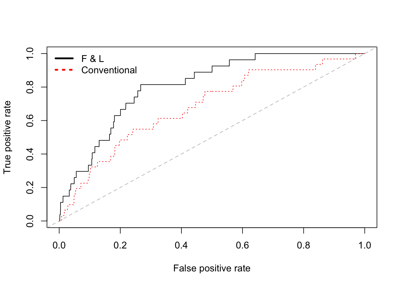
Let’s compare (1) a model with F&L’s favorite variables and (2) a model with conventional variables
# A model that includes F & L's favorite variables only
mod.fl <- glm(onset ~
                gdpenl + lpopl1 + lmtnest + Oil + nwstate,
              family = binomial(link = logit),
              data = train)

# A model that includes conventional independent variables only

mod.co <- glm(onset ~
                warl + ncontig + instab + polity2l +
                ethfrac + relfrac,
              family = binomial(link = logit),
              data = train)

stargazer(mod.fl, mod.co, type = "text")
##
## ==============================================
##                       Dependent variable:
##                   ----------------------------
##                              onset
##                        (1)            (2)
## ----------------------------------------------
## gdpenl              -0.280***
##                      (0.074)
##
## lpopl1               0.261***
##                      (0.071)
##
## lmtnest              0.200**
##                      (0.097)
##
## Oil                  0.696**
##                      (0.318)
##
## nwstate              1.519***
##                      (0.382)
##
## warl                                -0.552
##                                     (0.392)
##
## ncontig                             0.684**
##                                     (0.289)
##
## instab                              0.636**
##                                     (0.282)
##
## polity2l                            -0.012
##                                     (0.017)
##
## ethfrac                            1.233***
##                                     (0.437)
##
## relfrac                             -0.567
##                                     (0.555)
##
## Constant            -6.603***      -4.660***
##                      (0.726)        (0.275)
##
## ----------------------------------------------
## Observations          4,985          5,022
## Log Likelihood       -378.088      -397.515
## Akaike Inf. Crit.    768.175        809.030
## ==============================================
## Note:              *p<0.1; **p<0.05; ***p<0.01
# F & L
pred.fl <- predict(mod.fl, newdata = test, type = "response")
eval <- data.frame(cbind(pred.fl, test $ onset)); eval <- na.omit(eval)
colnames(eval) <- c("pred.fl", "onset")
prediction.fl <- prediction(eval$pred.fl, eval$ onset)
perf.fl <- performance(prediction.fl, "tpr", "fpr")

# Conventional
pred.co <- predict(mod.co, newdata = test, type = "response")
eval <- data.frame(cbind(pred.co, test $ onset)); eval <- na.omit(eval)
colnames(eval) <- c("pred.co", "onset")
prediction.co <- prediction(eval$pred.co, eval$onset)
perf.co <- performance(prediction.co, "tpr", "fpr")


# pdf("roc3.pdf")
{plot(perf.fl)  # model 1
abline(a = 0, b = 1, lty = "dashed", col="gray")
plot(perf.co, add = TRUE, col = "red", lty = "dotted")
legend("topleft",
       c("F & L","Conventional"),
       col = c("black","red"),
       cex=1, lwd=3, lty = c("solid", "dotted"), bty="n")}
# dev.off()
AUC
AUC (Area Under the ROC Curve) is obtained with the performance function with some options. Recall that AUC is between 0 and 1 (the higher, the better).
# Model 1
performance(prediction.fl1, "auc")@y.values
## [[1]]
## [1] 0.8106935
# Model 3
performance(prediction.fl3, "auc")@y.values
## [[1]]
## [1] 0.8209558
# F&L
performance(prediction.fl, "auc")@y.values
## [[1]]
## [1] 0.8077666
# Conventional
performance(prediction.co, "auc")@y.values
## [[1]]
## [1] 0.6837929
# Comparing the AUC scores, model 3 is slightly better than
# model 1, and both are better than the latter two
What would happen if we run a constant-only model, and obtain a ROC curve and AUC ?
mod.0 <- glm(onset ~ 1,
              family = binomial(link = logit),
              data = train)

stargazer(mod.0, type = "text")
##
## =============================================
##                       Dependent variable:
##                   ---------------------------
##                              onset
## ---------------------------------------------
## Constant                   -4.134***
##                             (0.113)
##
## ---------------------------------------------
## Observations                 5,076
## Log Likelihood             -411.386
## Akaike Inf. Crit.           824.773
## =============================================
## Note:             *p<0.1; **p<0.05; ***p<0.01
# ROC curve
pred.0 <- predict(mod.0, newdata = test, type = "response")
eval <- data.frame(cbind(pred.0, test $ onset)); eval <- na.omit(eval)
colnames(eval) <- c("pred.0", "onset")
prediction.0 <- prediction(eval$pred.0, eval$ onset)
perf.0 <- performance(prediction.0, "tpr", "fpr")

plot(perf.0)
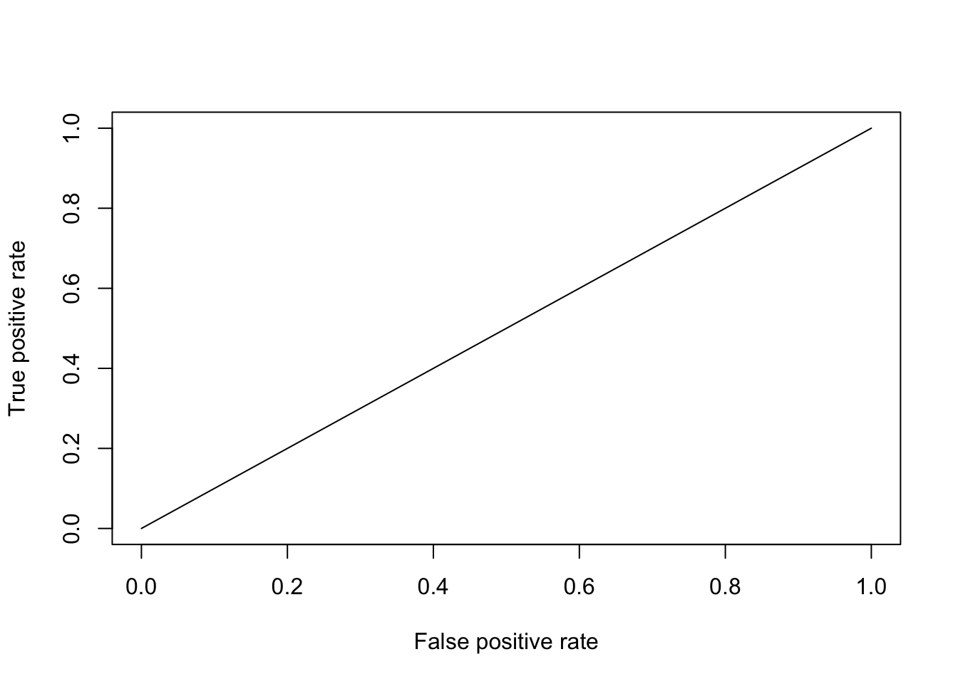 The ROC curve will be a 45-degree line. No matter what threshold we use, the PCP doesn’t change
hitmiss(mod.0)
## Classification Threshold = 0.5
##         y=0 y=1
## yhat=0 4996  80
## yhat=1    0   0
## Percent Correctly Predicted = 98.42%
## Percent Correctly Predicted = 100%, for y = 0
## Percent Correctly Predicted = 0%  for y = 1
## Null Model Correctly Predicts 98.42%

## [1]  98.42396 100.00000   0.00000
hitmiss(mod.0, k = 0.2)
## Classification Threshold = 0.2
##         y=0 y=1
## yhat=0 4996  80
## yhat=1    0   0
## Percent Correctly Predicted = 98.42%
## Percent Correctly Predicted = 100%, for y = 0
## Percent Correctly Predicted = 0%  for y = 1
## Null Model Correctly Predicts 98.42%

## [1]  98.42396 100.00000   0.00000
hitmiss(mod.0, k = 0.4)
## Classification Threshold = 0.4
##         y=0 y=1
## yhat=0 4996  80
## yhat=1    0   0
## Percent Correctly Predicted = 98.42%
## Percent Correctly Predicted = 100%, for y = 0
## Percent Correctly Predicted = 0%  for y = 1
## Null Model Correctly Predicts 98.42%

## [1]  98.42396 100.00000   0.00000
hitmiss(mod.0, k = 0.6)
## Classification Threshold = 0.6
##         y=0 y=1
## yhat=0 4996  80
## yhat=1    0   0
## Percent Correctly Predicted = 98.42%
## Percent Correctly Predicted = 100%, for y = 0
## Percent Correctly Predicted = 0%  for y = 1
## Null Model Correctly Predicts 98.42%

## [1]  98.42396 100.00000   0.00000
hitmiss(mod.0, k = 0.8)
## Classification Threshold = 0.8
##         y=0 y=1
## yhat=0 4996  80
## yhat=1    0   0
## Percent Correctly Predicted = 98.42%
## Percent Correctly Predicted = 100%, for y = 0
## Percent Correctly Predicted = 0%  for y = 1
## Null Model Correctly Predicts 98.42%

## [1]  98.42396 100.00000   0.00000
# AUC will be equal to 0.5

performance(prediction.0, "auc")@y.values
## [[1]]
## [1] 0.5
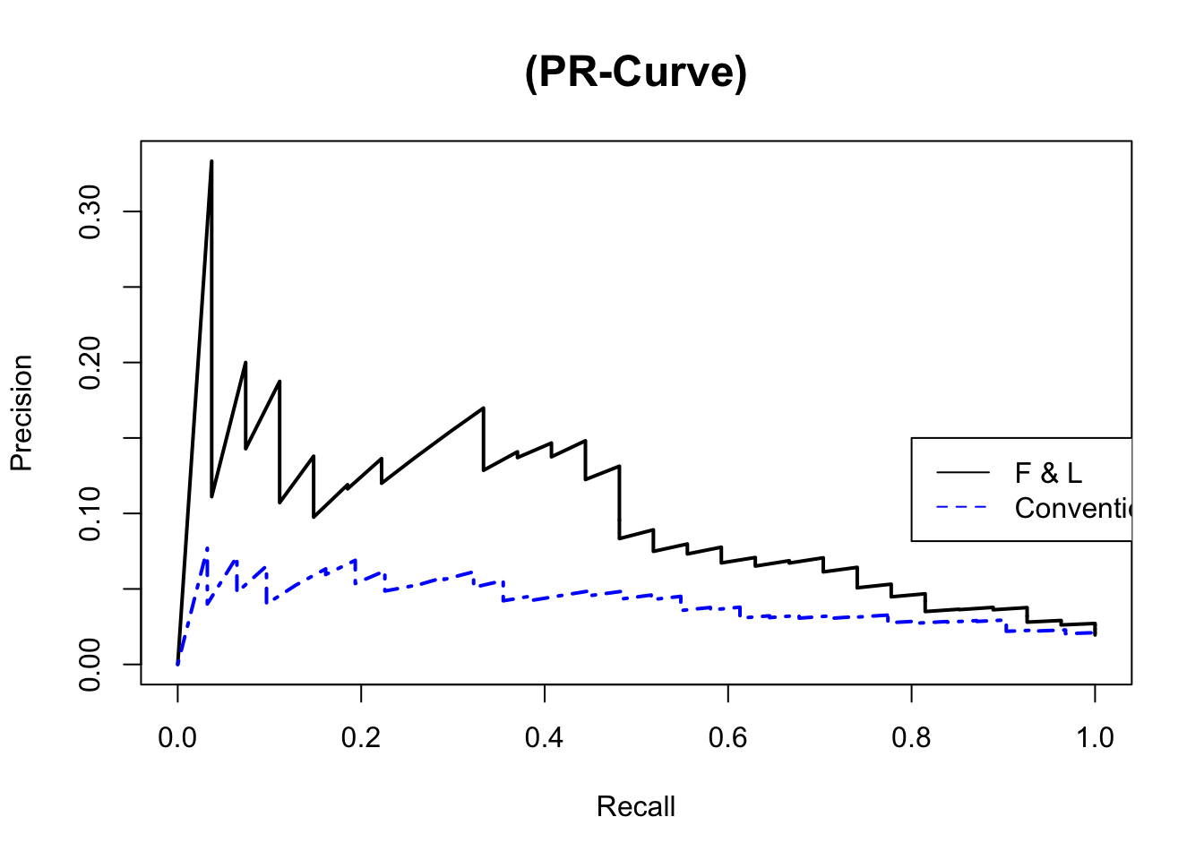
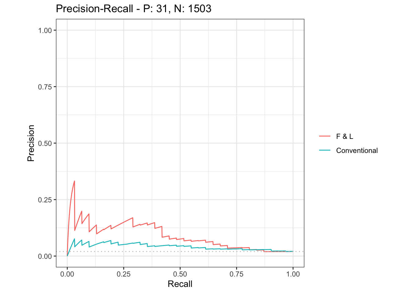
Precision Recall curve (PR curve)
Here is a PR curve function I wrote, you can just use it to plot
rocdf <- function(pred, obs, data=NULL, type=NULL) {
  library(ROCR)
  if (!is.null(data)) {
    pred <- eval(substitute(pred), envir=data)
    obs  <- eval(substitute(obs), envir=data)
  }
  rocr_xy <- switch(type, roc=c("tpr", "fpr"), pr=c("prec", "rec"))
  rocr_df <- prediction(pred, obs)
  rocr_pr <- performance(rocr_df, rocr_xy[1], rocr_xy[2])
  xy <- data.frame(rocr_pr@x.values[[1]], rocr_pr@y.values[[1]])
  if (type=="pr") {
    xy[1, 2] <- 0   }
  colnames(xy) <- switch(type, roc=c("tpr", "fpr"), pr=c("rec", "prec"))
  return(xy)
}

# the "conventional variables only" model
eval.co <- data.frame(cbind(pred.co, test $ onset)); eval.co <- na.omit(eval.co)
colnames(eval.co) <- c("pred.co", "onset")

eval.fl3 <- data.frame(cbind(pred.fl3, test $ onset)); eval.fl3 <- na.omit(eval.fl3)
colnames(eval.fl3) <- c("pred.fl3", "onset")

fl <- rocdf(as.numeric(unlist(eval.fl3$pred.fl3)), # column
            as.numeric(unlist(eval.fl3$onset)), type="pr")

base <-rocdf(as.numeric(unlist(eval.co$pred.co)),
               as.numeric(unlist(eval.co$onset)) , type="pr")

# pdf(file="Week20/figs/PR_fl3_co.pdf",width=10, height=8)
{plot(fl$rec, fl$prec, type="l", lty=1, col="black", lwd=2, main="(PR-Curve)", #family="Garamond",
     cex.axis=1, cex.lab=1, cex.main=1.5,
     xlab="Recall", ylab="Precision")
# lines(china.svm[, 1], china.svm[, 2], type="l", lty=2, col='red', lwd=2)
# lines(china.rf[, 1], china.rf[, 2], type="l", lty=3, col='blue', lwd=2)
lines(base$rec, base$prec, type="l", lty=4, col="blue", lwd=2) # burlywood4
legend(0.8, 0.15, legend=c("F & L","Conventional"), lty=1:4, col=c('black',"blue"))}
# dev.off()
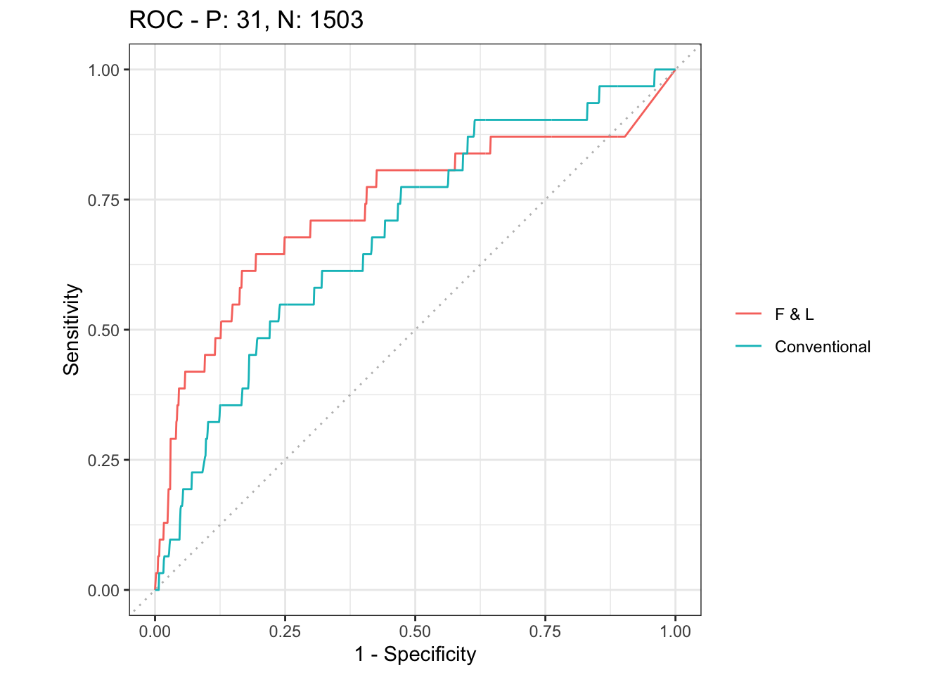
Alternatively, we can use the package precrec to plot ROC and PR curves
library(precrec)
library(ggplot2)
library(grid)
library(tidyverse)

# First, we make sure that evaluation tables all have the same number of observations. To do so, we merge the table together.

eval.fl3 <- data.frame(cbind(pred.fl3, test $ onset))
colnames(eval.fl3) <- c("pred.fl3", "onset")
eval.fl3$merger <- 1:nrow(eval.fl3)

eval.co <- data.frame(cbind(pred.co, test $ onset))
colnames(eval.co) <- c("pred.co", "onset")
eval.co$merger <- 1:nrow(eval.co)

eval.fl3.co <- left_join(eval.fl3, eval.co, by = c("merger" = "merger", "onset" ="onset"))

# Then, we specify scores (scores usually mean the predicted values) and labels (labels typically mean the actual data).
scores1 = eval.fl3.co$pred.fl3; labels1 = eval.fl3.co$onset
scores2 = eval.fl3.co$pred.co; labels2 = eval.fl3.co$onset
scores <- join_scores(scores1, scores2)
labels <- join_labels(labels1, labels2)

# We can explicitly specify model names
msmdat2 <- mmdata(scores, labels, modnames = c("F & L", "Conventional"))

mscurves <- evalmod(msmdat2)
# NA rows will be dropped by the autoplot function
# pdf(file="Week20/figs/ROC_fl3_co.pdf",width=10, height=8)
ggplot2::autoplot(mscurves, show_legend = T, curvetype = "ROC") # ROC curve
## Warning in ggplot2::fortify(object, raw_curves = raw_curves, reduce_points = reduce_points): Arguments in `...` must be used.
## ✖ Problematic argument:
## • raw_curves = raw_curves
## ℹ Did you misspell an argument name?
# dev.off()

# pdf(file="Week20/figs/PR_fl3_co2.pdf",width=10, height=8)
ggplot2::autoplot(mscurves, show_legend = T, curvetype = "PRC") # PR curve
## Warning in ggplot2::fortify(object, raw_curves = raw_curves, reduce_points = reduce_points): Arguments in `...` must be used.
## ✖ Problematic argument:
## • raw_curves = raw_curves
## ℹ Did you misspell an argument name?
# dev.off()
# Codebook for the Fearon & Laitin data set -------------------------------

# ccode         COW country code
# country       country name
# cname         abbreviated country name
# cmark         1 for first in each country series
# year          start year of war/conflict
# wars          # wars in progress in country year
# war           1 if war ongoing in country year
# warl          lagged war, w/ 0 for start of country series
# onset         1 for civil war onset
# ethonset      1 if onset = 1 & ethwar ~= 0
# durest        estimated war duration
# aim           1 = rebels aim at center, 3 = aim at exit or autonomy, 2 = mixed or ambig.
# casename      Id for case, usually name of rebel group(s)
# ended         war ends = 1, 0 = ongoing
# ethwar        0 = not ethnic, 1 = ambig/mixed, 2 = ethnic
# waryrs        war years for each onset
# pop           population, in 1000s
# lpop          log of pop
# polity2       revised polity score
# gdpen         gdp/pop based on pwt5.6, wdi2001,cow energy data
# gdptype       source/type of gdp/pop estimate
# gdpenl        lagged gdpenl, except for first in country series
# lgdpenl1      log of lagged gdpen
# lpopl1        log population, lagged except for first in country series
# region        country's region, based on MAR project
# western       Dummy for Western Democracies & Japan
# eeurop        Dummy for Eastern Europe
# lamerica      Dummy for Latin America
# ssafrica      Dummy for Sub-Saharan Africa
# asia          Dummy for Asia (-Japan)
# nafrme        Dummy for North Africa/Middle East
# colbrit       Former British colony
# colfra        former French colony
# mtnest        Estimated % mountainous terrain
# lmtnest       log of mtnest
# elevdiff      high - low elevation, in meters
# Oil           > 1/3 export revenues from fuels
# ncontig       noncontiguous state
# ethfrac       ethnic frac. based on Soviet Atlas, plus est's for missing in 1964
# ef            ethnic fractionalization based on Fearon 2002 APSA paper
# plural        share of largest ethnic group (Fearon 2002 APSA)
# second        share of 2nd largest ethnic group (Fearon 2002 APSA)
# numlang       # languages in Ethnologue > min(1% pop, 1mill)
# relfrac       religious fractionalization
# plurrel       size of largest confession
# minrelpc      size of second largest confession
# muslim        % muslim
# nwstate       1 in 1st 2 years of state's existence
# polity2l      lagged polity2, except 1st in country series
# instab        > 2 change in Polity measure in last 3 yrs
# anocl         lagged anocracy (-6 < polity2l < 6)
# deml          lagged democracy (polity2l > 5)
# empethfrac    ethfrac coded for colonial empires
# empwarl       warl coded for data with empires
# emponset      onset coded for data with empires
# empgdpenl     gdpenl coded for empires data
# emplpopl      lpopl coded for empires data
# emplmtnest    lmtnest coded for empires data
# empncontig    ncontig coded for empires
# empolity2l    polity2l adjusted for empires (see fn38 in paper)
# sdwars        # Sambanis/Doyle civ wars in progress
# sdonset       onset of Sambanis/Doyle war
# colwars       # Collier/Hoeffler wars in progress
# colonset      onset of Collier/Hoeffler war
# cowwars       # COW civ wars in progress
# cowonset      onset of COW civ war
# cowwarl       1 if COW war ongoing in last period
# sdwarl        1 if S/D war ongoing in last period
# colwarl       1 if C/H war ongoing in last period