Point Estimates and CIs
rm(list=ls(all=TRUE))
cat("\014")
The source qmd file can be found here
Download the data
- If you haven’t done so already, create a folder named “POLI502” somewhere on your computer (could be on your desktop, documents folder, etc.)
- Download all the files you need for today from Blackboard and save them in the folder (world.csv).
- Load packages we use
library(ggplot2)
library(magrittr)
library(tidyverse) # manipulate data
1. Constructing a 95% confidence interval
Whenever we report the results of our statistical analysis, we should report our uncertainty estimates. That is, we report the amount of error that we think exists in our inference. Put differently, we report how much confidence we can have about our estimate.
As we learned in the lecture, we do this in a way that is probably not very intuitive to you. We do NOT say things like, “we are 30% confident about this estimate”, or “we are 95% confident about that estimate”. Instead, what we do is the following.
For a given level of confidence (conventionally, it is 95%), we construct and report an interval of values that we think contains the true & unknown population parameter. This interval is called a confidence interval. If we construct this interval for a 95% confidence level, we call it a 95% confidence interval. (You might wonder why 95%. As I said, there is no good reason. We use 95% just because it is the convention.)
So, in reporting our estimate of the mean of a variable, we report the sample mean (point estimate) as well as the associated 95% confidence interval of the mean (interval estimate).
To construct a 95% confidence interval (CI), we need two things:
-
We first need the point estimate. When estimating the population mean, the sample mean is our point estimate (our “best” guess). The point estimate will be used as the center of the confidence interval.
-
Second, we need a standard error (SE) of the estimate. With these two,
- The lower bound of the 95% CI is: point estimate - 2 * SE
- The upper bound of the 95% CI is: point estimate + 2 * SE (We sometimes use 1.96 instead of 2 to be more precise.)
As we discussed in the lecture, this is the interval that would contain the true population parameter 95% of the time if we were to repeat the sampling process many, many times. This is how we interepret confidence intervals. This is how we report our uncertainty.
Let’s try constructing a 95% confidence interval of the mean for a numerical variable in the “world” data set.
Load the world data set
world.data <- read.csv("world.csv")
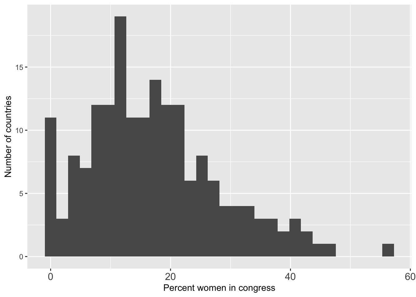
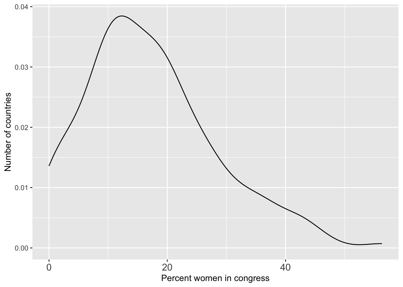
We will analyze the women09 variable, which measures the percentage of female congresspersons in lower house of parliament in 2009.
Numerical and graphical summaries
Numerical summaries
summary(world.data $ women09)
##    Min. 1st Qu.  Median    Mean 3rd Qu.    Max.    NA's
##    0.00    9.70   15.55   17.18   22.95   56.30      11
world.data $ women09 %>% class
## [1] "numeric"
is.na(world.data$women09)
##   [1] FALSE FALSE FALSE FALSE FALSE FALSE FALSE FALSE FALSE FALSE FALSE FALSE
##  [13] FALSE FALSE FALSE FALSE FALSE FALSE FALSE FALSE FALSE FALSE FALSE FALSE
##  [25]  TRUE FALSE FALSE FALSE FALSE FALSE FALSE FALSE FALSE FALSE FALSE FALSE
##  [37] FALSE FALSE  TRUE  TRUE FALSE FALSE FALSE FALSE FALSE FALSE FALSE FALSE
##  [49] FALSE FALSE FALSE FALSE FALSE FALSE FALSE FALSE FALSE  TRUE FALSE FALSE
##  [61] FALSE FALSE FALSE FALSE FALSE FALSE FALSE FALSE FALSE  TRUE FALSE FALSE
##  [73] FALSE FALSE FALSE FALSE FALSE FALSE FALSE FALSE FALSE FALSE FALSE FALSE
##  [85] FALSE FALSE FALSE FALSE FALSE FALSE FALSE FALSE FALSE FALSE FALSE FALSE
##  [97] FALSE FALSE FALSE FALSE FALSE FALSE  TRUE FALSE FALSE FALSE FALSE FALSE
## [109] FALSE FALSE FALSE FALSE FALSE  TRUE FALSE FALSE FALSE FALSE  TRUE FALSE
## [121] FALSE FALSE FALSE FALSE FALSE FALSE FALSE FALSE FALSE FALSE FALSE FALSE
## [133] FALSE FALSE FALSE FALSE FALSE FALSE FALSE FALSE FALSE FALSE FALSE FALSE
## [145] FALSE FALSE FALSE FALSE FALSE FALSE FALSE FALSE FALSE FALSE FALSE FALSE
## [157] FALSE FALSE FALSE FALSE FALSE FALSE FALSE FALSE FALSE  TRUE FALSE FALSE
## [169] FALSE FALSE FALSE FALSE FALSE FALSE FALSE FALSE FALSE FALSE FALSE FALSE
## [181] FALSE FALSE FALSE FALSE FALSE FALSE  TRUE FALSE  TRUE FALSE FALSE
world.data $ women09 %>% na.omit %>% mean
## [1] 17.17722
sd(world.data $ women09, na.rm = TRUE)
## [1] 11.05299
Histogram:
g <- ggplot(world.data, aes(x = women09))
g <- g + geom_histogram()
g <- g + theme(axis.text.x = element_text(size = 12))
g <- g + xlab("Percent women in congress")
g <- g + ylab("Number of countries")
g
## `stat_bin()` using `bins = 30`. Pick better value with `binwidth`.

## Warning: Removed 11 rows containing non-finite outside the scale range
## (`stat_bin()`).

#same thing, just clearer in your code
g <- ggplot(world.data, aes(x = women09)) +
  geom_histogram() + #geom_histogram(binwidth = 1)
  theme(axis.text.x = element_text(size = 12)) +
  xlab("Percent women in congress") + ylab("Number of countries")
g
## `stat_bin()` using `bins = 30`. Pick better value with `binwidth`.

## Warning: Removed 11 rows containing non-finite outside the scale range
## (`stat_bin()`).
Density plot (smoothed histogram)
g <- ggplot(world.data, aes(x = women09))
g <- g + geom_density()
g <- g + theme(axis.text.x = element_text(size = 12))
g <- g + xlab("Percent women in congress")
g <- g + ylab("Number of countries")
g
## Warning: Removed 11 rows containing non-finite outside the scale range
## (`stat_density()`).
Constructing a 95% confidence interval
First, we need the point estimate (center of the 95% CI)
mean(world.data $ women09, na.rm = TRUE)
## [1] 17.17722
Let’s store this into an object, so we can use it later.
pe <- mean(world.data $ women09, na.rm = TRUE)
Second, we need to obtain the standard error (SE). Recall that the SE for mean is obtained by SD divided by sqrt(n), so we need to obtain SD (standard deviation) and n (sample size).
SD: we already did this above. Let’s store it into an object.
sd <- sd(world.data $ women09, na.rm = TRUE)
n: the sample size is the number of observations included in this sample. We can use the length function to find out, but be very careful: we have missing values.
So, if we do this
length(world.data $ women09)
## [1] 191
R tells us that there are 191 values. However, we don’t actually have 191 values because some of them are NAs. As we saw above,
summary(world.data $ women09)
##    Min. 1st Qu.  Median    Mean 3rd Qu.    Max.    NA's
##    0.00    9.70   15.55   17.18   22.95   56.30      11
There are 11 NA’s in the data set, so we actually have 191-11 = 180 observations. One way to obtain the correct sample size (n = 180) is to combine the is.na function.
The is.na function returns a logical value, TRUE or FALSE. For example,
x <- c(4, NA, 1, -2, NA, 2)

is.na(x)
## [1] FALSE TRUE FALSE FALSE TRUE FALSE
R says that the second and the fifth elements of this x vector are TRUE, meaning that they are NAs. Combining this is.na function and the square brackets [ ], we can do things like the following:
x[ is.na(x) == FALSE ]
## [1] 4 1 -2 2
Remember that square brackets [ ] let us extract a subset of a vector or a matrix that satisfies some conditions. In the example above, we extracted a subset of x that satisfies the condition is.na(x)==FALSE. (Note that we need two equal signs because we are specifying a condition.) Alternatively, we can write the following to get the same outcome.
x[ is.na(x) != TRUE ]
## [1] 4 1 -2 2
We can see that we extracted the non-missing values of the x vector. Then, we can find the number of non-missing elements in x, as follows:
length( x[ is.na(x) == FALSE ] )
## [1] 4
Or you can simply use “!” this instead.
x[!is.na(x)]
## [1] 4 1 -2 2
x[!is.na(x)] %>% length
## [1] 4
which is different from
length(x)
## [1] 6
Going back to the women09 variable, the sample size can be obtained by:
length( world.data $ women09[is.na(world.data $ women09) == FALSE] )
## [1] 180
length( world.data $ women09[!is.na(world.data $ women09)] )
## [1] 180
n <- length( world.data $ women09[is.na(world.data $ women09) == FALSE] )
Let’s store this into an object:
n <- world.data $ women09[is.na(world.data $ women09) == FALSE] %>% length()

# Then, the standard error (SE) is SD/sqrt(n), so

sd/sqrt(n)
## [1] 0.8238416
# we will store this into an object

se <- sd/sqrt(n)
To summarize, we need the following:
# 1: Point estimate
pe <- mean(world.data $ women09, na.rm = TRUE)

# 2: Standard error
sd <- sd(world.data $ women09, na.rm = TRUE)
n <- length( world.data $ women09[is.na(world.data $ women09) == FALSE] )
se <- sd/sqrt(n)


# Finally, we construct a 95% confidence interval by identifying the
# lower and upper bounds

pe - 2 * se   # Lower bound
## [1] 15.52954
pe + 2 * se # Upper bound
## [1] 18.82491
So, we report the results verbally, as follows: The mean of women09 is 17.18 % with a 95% confidence interval of [15.53, 18.82]. Or we can report them directly using R command here, [15.529539, 18.8249054]
2. Create a subset of a data set
Sometimes it makes sense to create a smaller data set that contains a subset of observations. For example, we have seen above that missing values can make our calculation unnecessarily complicated. We can avoid this by working with a smaller data set that excludes observations with missing values.
We have learned in the past weeks how to create a subset of a data set using square bracket. For example,
world.data %>% dim
## [1] 191 62
world.data[ 2:5, 1:4 ]
##   country       colony confidence decentralization
## 2 Albania Soviet Union   49.33593             0.74
## 3 Algeria       France   52.05573               NA
## 4 Andorra        Spain         NA               NA
## 5  Angola     Portugal         NA               NA
The code above tells R to extract rows 2 through 5 (2:5) and columns 1 through 4 (1:4) of the world.data.
The numbers BEFORE the comma specify what rows you want to extract and the numbers AFTER the comma specify what columns you want to extract.
We can also do things like
world.data[ 1:2, ] %>% head
##       country       colony confidence decentralization dem_other dem_other5
## 1 Afghanistan           UK         NA               NA      10.5        10%
## 2     Albania Soviet Union   49.33593             0.74      63.0 Approx 60%
##   democ_regime district_size3 durable effectiveness      enpp_3         eu
## 1           No  single member       4      13.71158             Not member
## 2          Yes                      3      35.46099 1-3 parties Not member
##   fhrate04_rev fhrate08_rev frac_eth frac_eth3 free_business free_corrupt
## 1          2.5            3   0.7693      High            NA           NA
## 2            5            8   0.2204       Low            68           34
##   free_finance free_fiscal free_govspend free_invest free_labor free_monetary
## 1           NA          NA            NA          NA         NA            NA
## 2           70        92.6          74.2          70       52.1          78.7
##   free_overall free_property free_trade gdp08 gdp_10_thou gdp_cap2 gdp_cap3
## 1           NA            NA         NA  30.6          NA
## 2           66            35       85.8  24.3      0.1535      Low   Middle
##   gdppcap08 gender_equal3 gini04 gini08  hi_gdp indy       oecd  old2006
## 1        NA                   NA     NA         1919 Not member       NA
## 2      7715                 28.2   31.1 Low GDP 1991 Not member 8.479821
##    old2003     pmat12_3   pop03 pop08    pop08_3          popcat3 pr_sys
## 1       NA                   NA  27.4 >=16.8 mil Moderate (1-29m)     No
## 2 7.278363 Low post-mat 3169064   3.1  <=4.3 mil Moderate (1-29m)     No
##   protact3        regime_type3      region sources typerel unions urban03
## 1                 Dictatorship Middle East      NA  Muslim     NA      NA
## 2 Moderate Parliamentary democ  C&E Europe      NA  Muslim     NA  44.239
##   urban06 vi_rel3 votevap00s women05 women09 womyear       womyear2  yng2003
## 1   23.28                 NA      NA    27.7      NA                      NA
## 2   46.14  20-50%      59.56     6.4    16.4    1920 1944 or before 27.34834
##    young06
## 1       NA
## 2 26.35428
# Rows 1 through 2 for ALL columns,
world.data[ , 1:2 ] %>% head
##             country       colony
## 1       Afghanistan           UK
## 2           Albania Soviet Union
## 3           Algeria       France
## 4           Andorra        Spain
## 5            Angola     Portugal
## 6 Antigua & Barbuda           UK
# All rows for columns 1 and 2.

# We can provide some logical conditions instead of row/column numbers
# as follows:

world.data[ world.data $ region == "N. America" ,  1:5 ]
##           country colony confidence decentralization dem_other
## 31         Canada     UK   58.20387             2.45       100
## 112        Mexico  Spain   26.04039             2.04       100
## 181 United States     UK   61.78521             2.20       100
# Or you can use dplyr to achieve the same outcome:
world.data %>%
  filter(region == "N. America")%>%
  select(1:5)
##         country colony confidence decentralization dem_other
## 1        Canada     UK   58.20387             2.45       100
## 2        Mexico  Spain   26.04039             2.04       100
## 3 United States     UK   61.78521             2.20       100
# This extracts all the rows (= all the countries) that satisfy the
# condition: world.data $ region == "N. America"
Combining what we have learned so far, we can create a smaller data set that excludes all countries for which women09 is missing, as follows:
wd.women09 <- world.data[ is.na(world.data $ women09) == FALSE , ]
head(wd.women09)
##             country       colony confidence decentralization dem_other
## 1       Afghanistan           UK         NA               NA      10.5
## 2           Albania Soviet Union   49.33593             0.74      63.0
## 3           Algeria       France   52.05573               NA      40.8
## 4           Andorra        Spain         NA               NA     100.0
## 5            Angola     Portugal         NA               NA      40.8
## 6 Antigua & Barbuda           UK         NA               NA      87.5
##   dem_other5 democ_regime    district_size3 durable effectiveness      enpp_3
## 1        10%           No     single member       4      13.71158
## 2 Approx 60%          Yes                         3      35.46099 1-3 parties
## 3 Approx 40%           No 6 or more members       5      32.62411
## 4       100%          Yes                        NA      78.72340
## 5 Approx 40%           No                         3      19.14894
## 6 Approx 90%          Yes     single member      NA      59.81088 1-3 parties
##           eu fhrate04_rev fhrate08_rev frac_eth frac_eth3 free_business
## 1 Not member          2.5            3   0.7693      High            NA
## 2 Not member            5            8   0.2204       Low          68.0
## 3 Not member          2.5            3   0.3394    Medium          71.2
## 4 Not member    Most free           12   0.7139      High            NA
## 5 Not member          2.5            3   0.7867      High          43.4
## 6 Not member            6           10   0.1643       Low            NA
##   free_corrupt free_finance free_fiscal free_govspend free_invest free_labor
## 1           NA           NA          NA            NA          NA         NA
## 2           34           70        92.6          74.2          70       52.1
## 3           32           30        83.5          73.4          45       56.4
## 4           NA           NA          NA            NA          NA         NA
## 5           19           40        85.1          62.8          35       45.2
## 6           NA           NA          NA            NA          NA         NA
##   free_monetary free_overall free_property free_trade gdp08 gdp_10_thou
## 1            NA           NA            NA         NA  30.6          NA
## 2          78.7         66.0            35       85.8  24.3      0.1535
## 3          77.2         56.9            30       70.7 276.0      0.1785
## 4            NA           NA            NA         NA    NA          NA
## 5          62.6         48.4            20       70.4 106.3      0.0857
## 6            NA           NA            NA         NA    NA      1.0449
##   gdp_cap2 gdp_cap3 gdppcap08 gender_equal3 gini04 gini08   hi_gdp indy
## 1                          NA                   NA     NA          1919
## 2      Low   Middle      7715                 28.2   31.1  Low GDP 1991
## 3      Low   Middle      8033                 35.3   35.3  Low GDP 1962
## 4                          NA                   NA     NA          1278
## 5      Low   Middle      5899                   NA     NA  Low GDP 1975
## 6     High     High        NA                   NA     NA High GDP 1981
##         oecd  old2006  old2003     pmat12_3    pop03 pop08    pop08_3
## 1 Not member       NA       NA                    NA  27.4 >=16.8 mil
## 2 Not member 8.479821 7.278363 Low post-mat  3169064   3.1  <=4.3 mil
## 3 Not member 4.578136 4.045199              31832610  34.4 >=16.8 mil
## 4 Not member       NA       NA                 66000    NA
## 5 Not member 2.450295 2.930542              13522110  18.0 >=16.8 mil
## 6 Not member       NA 8.186610                 78580    NA
##            popcat3 pr_sys protact3        regime_type3      region sources
## 1 Moderate (1-29m)     No                 Dictatorship Middle East      NA
## 2 Moderate (1-29m)     No Moderate Parliamentary democ  C&E Europe      NA
## 3 Moderate (1-29m)    Yes                 Dictatorship      Africa      NA
## 4 Small (under 1m)     No          Parliamentary democ   W. Europe      NA
## 5 Moderate (1-29m)    Yes                 Dictatorship      Africa      NA
## 6 Small (under 1m)     No          Parliamentary democ  S. America      NA
##          typerel unions urban03 urban06 vi_rel3 votevap00s women05 women09
## 1         Muslim     NA      NA   23.28                 NA      NA    27.7
## 2         Muslim     NA 44.2390   46.14  20-50%      59.56     6.4    16.4
## 3         Muslim     NA 58.8302   63.94    >50%         NA      NA     7.7
## 4 Roman Catholic     NA 91.7404   90.28              20.95    14.3    35.7
## 5 Roman Catholic     NA 36.1806   53.96                 NA      NA    37.3
## 6     Protestant     NA 37.7566   39.60              76.34    10.5    10.5
##   womyear       womyear2  yng2003  young06
## 1      NA                      NA       NA
## 2    1920 1944 or before 27.34834 26.35428
## 3    1962     After 1944 33.91887 28.94154
## 4    1973     After 1944       NA       NA
## 5    1975     After 1944 47.62524 46.32196
## 6    1951     After 1944 20.66509       NA
wd.women09 <- world.data %>% filter(!is.na(women09))
head(wd.women09)
##             country       colony confidence decentralization dem_other
## 1       Afghanistan           UK         NA               NA      10.5
## 2           Albania Soviet Union   49.33593             0.74      63.0
## 3           Algeria       France   52.05573               NA      40.8
## 4           Andorra        Spain         NA               NA     100.0
## 5            Angola     Portugal         NA               NA      40.8
## 6 Antigua & Barbuda           UK         NA               NA      87.5
##   dem_other5 democ_regime    district_size3 durable effectiveness      enpp_3
## 1        10%           No     single member       4      13.71158
## 2 Approx 60%          Yes                         3      35.46099 1-3 parties
## 3 Approx 40%           No 6 or more members       5      32.62411
## 4       100%          Yes                        NA      78.72340
## 5 Approx 40%           No                         3      19.14894
## 6 Approx 90%          Yes     single member      NA      59.81088 1-3 parties
##           eu fhrate04_rev fhrate08_rev frac_eth frac_eth3 free_business
## 1 Not member          2.5            3   0.7693      High            NA
## 2 Not member            5            8   0.2204       Low          68.0
## 3 Not member          2.5            3   0.3394    Medium          71.2
## 4 Not member    Most free           12   0.7139      High            NA
## 5 Not member          2.5            3   0.7867      High          43.4
## 6 Not member            6           10   0.1643       Low            NA
##   free_corrupt free_finance free_fiscal free_govspend free_invest free_labor
## 1           NA           NA          NA            NA          NA         NA
## 2           34           70        92.6          74.2          70       52.1
## 3           32           30        83.5          73.4          45       56.4
## 4           NA           NA          NA            NA          NA         NA
## 5           19           40        85.1          62.8          35       45.2
## 6           NA           NA          NA            NA          NA         NA
##   free_monetary free_overall free_property free_trade gdp08 gdp_10_thou
## 1            NA           NA            NA         NA  30.6          NA
## 2          78.7         66.0            35       85.8  24.3      0.1535
## 3          77.2         56.9            30       70.7 276.0      0.1785
## 4            NA           NA            NA         NA    NA          NA
## 5          62.6         48.4            20       70.4 106.3      0.0857
## 6            NA           NA            NA         NA    NA      1.0449
##   gdp_cap2 gdp_cap3 gdppcap08 gender_equal3 gini04 gini08   hi_gdp indy
## 1                          NA                   NA     NA          1919
## 2      Low   Middle      7715                 28.2   31.1  Low GDP 1991
## 3      Low   Middle      8033                 35.3   35.3  Low GDP 1962
## 4                          NA                   NA     NA          1278
## 5      Low   Middle      5899                   NA     NA  Low GDP 1975
## 6     High     High        NA                   NA     NA High GDP 1981
##         oecd  old2006  old2003     pmat12_3    pop03 pop08    pop08_3
## 1 Not member       NA       NA                    NA  27.4 >=16.8 mil
## 2 Not member 8.479821 7.278363 Low post-mat  3169064   3.1  <=4.3 mil
## 3 Not member 4.578136 4.045199              31832610  34.4 >=16.8 mil
## 4 Not member       NA       NA                 66000    NA
## 5 Not member 2.450295 2.930542              13522110  18.0 >=16.8 mil
## 6 Not member       NA 8.186610                 78580    NA
##            popcat3 pr_sys protact3        regime_type3      region sources
## 1 Moderate (1-29m)     No                 Dictatorship Middle East      NA
## 2 Moderate (1-29m)     No Moderate Parliamentary democ  C&E Europe      NA
## 3 Moderate (1-29m)    Yes                 Dictatorship      Africa      NA
## 4 Small (under 1m)     No          Parliamentary democ   W. Europe      NA
## 5 Moderate (1-29m)    Yes                 Dictatorship      Africa      NA
## 6 Small (under 1m)     No          Parliamentary democ  S. America      NA
##          typerel unions urban03 urban06 vi_rel3 votevap00s women05 women09
## 1         Muslim     NA      NA   23.28                 NA      NA    27.7
## 2         Muslim     NA 44.2390   46.14  20-50%      59.56     6.4    16.4
## 3         Muslim     NA 58.8302   63.94    >50%         NA      NA     7.7
## 4 Roman Catholic     NA 91.7404   90.28              20.95    14.3    35.7
## 5 Roman Catholic     NA 36.1806   53.96                 NA      NA    37.3
## 6     Protestant     NA 37.7566   39.60              76.34    10.5    10.5
##   womyear       womyear2  yng2003  young06
## 1      NA                      NA       NA
## 2    1920 1944 or before 27.34834 26.35428
## 3    1962     After 1944 33.91887 28.94154
## 4    1973     After 1944       NA       NA
## 5    1975     After 1944 47.62524 46.32196
## 6    1951     After 1944 20.66509       NA
# Then, the process of calculating the mean for women09 becomes a little
# bit simpler.

# 1: Point estimate
pe <- mean( wd.women09 $ women09 )

# 2: Standard error
sd <- sd( wd.women09 $ women09 )
n <- length( wd.women09 $ women09 )
se <- sd/sqrt(n)

pe          # Point estimate
## [1] 17.17722
pe - 2 * se # lower bound
## [1] 15.52954
pe + 2 * se # upper bound
## [1] 18.82491
# We get 17.18 with a 95% CI of [15.53, 18.82], just as before.
3. Re-labeling a factor variable
Let’s say we are interested in describing the gini08 variable for democracies and non-democracies using the democ_regime variable.
We have learned about the facet_wrap option previously. So, re-using the same commands, we can do
g <- ggplot(world.data, aes(x = gini08))
g <- g + geom_histogram()
g <- g + theme(axis.text.x = element_text(size = 12))
g <- g + xlab("Gini coefficient")
g <- g + ylab("Number of countries")
g <- g + facet_wrap( ~ democ_regime) # we can create separate histograms of gini08 for differenr regime types.
g
## `stat_bin()` using `bins = 30`. Pick better value with `binwidth`.

## Warning: Removed 64 rows containing non-finite outside the scale range
## (`stat_bin()`).
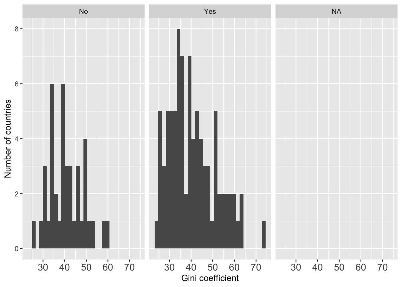
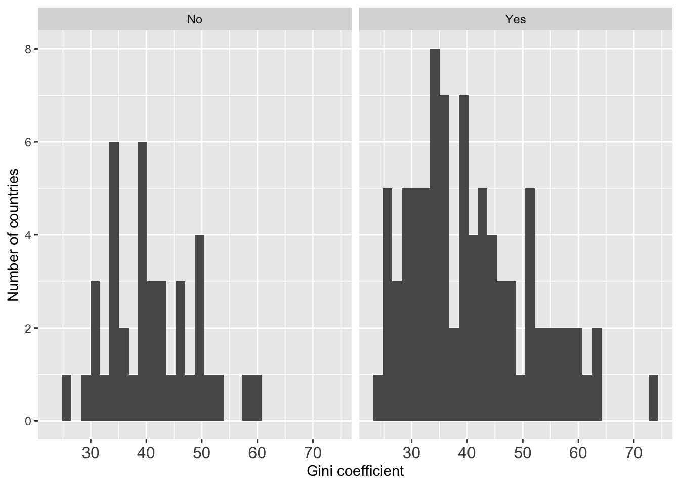
What’s a bit annoying about this graph is that we have a blank panel on the far right. This happens because there are observations where the democ_regime variable is missing. To remedy this, we need to create a smaller data set that excludes observations with missing values, just like we did above.
Another undesirable thing is that the graph titles are not very informative. We just see “No”, “Yes”, and “NA”, but readers wouldn’t know what they mean. It would be better if we label them so that readers can easily see what they mean. To do so, we need to re-label the factor variable, democ_regime.
Construct a smaller data set first:
wd.dem <- world.data[ is.na(world.data $ democ_regime) == FALSE , ]
wd.dem <- world.data %>% filter(!is.na(democ_regime)) # remove NAs


# If we create the same histograms with this smaller data set, we will
# no longer have a blank graph:

g <- ggplot(wd.dem, aes(x = gini08))
g <- g + geom_histogram()
g <- g + theme(axis.text.x = element_text(size = 12))
g <- g + xlab("Gini coefficient")
g <- g + ylab("Number of countries")
g <- g + facet_wrap( ~ democ_regime)
g
## `stat_bin()` using `bins = 30`. Pick better value with `binwidth`.

## Warning: Removed 62 rows containing non-finite outside the scale range
## (`stat_bin()`).
Let’s now re-label the factor variable,democ_regime.
We will do so by creating a new variable that is equal to the original democ_regime variable, except for the labels. The new variable should be coded as “Democracy” (rather than “Yes”) for democratic countries and “Autocracy” (rather than “No”) for non-democratic countries.
To create a new factor variable, we use the factor variable. Let’s call the new variable “democ”. We do the following.
wd.dem $ democ <- factor(wd.dem $ democ_regime,
                         levels = c("No", "Yes"),
                         labels = c("Autocracy", "Democracy")
                         )

# Then, if we create the histogram using the newly created factor:

g <- ggplot(wd.dem, aes(x = gini08))
g <- g + geom_histogram()
g <- g + theme(axis.text.x = element_text(size = 12))
g <- g + xlab("Gini coefficient")
g <- g + ylab("Number of countries")
g <- g + facet_wrap( ~ democ)
g + theme_bw() # I like a black-white theme more
## `stat_bin()` using `bins = 30`. Pick better value with `binwidth`.

## Warning: Removed 62 rows containing non-finite outside the scale range
## (`stat_bin()`).
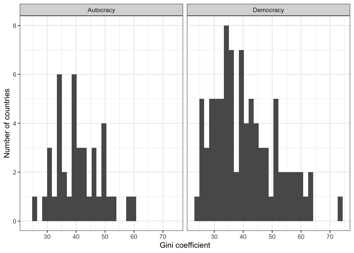
Now the titles are more informative. Hooray!
