Multiple Regression
Preparation
rm(list = ls())       # delete everything in the memory
library(foreign)      # for read.dta
library(ggplot2)      # for graphics
library(stargazer)    # Regression table
library(effects)
Learning objective:
We will learn four types of models here:
- Model with a dummy X
- Model with no X
- Model with a non-binary nominal X
- Model with an ordinal X
1. Model with a dummy variable
Load the Putnam 1994 data
pd <- read.csv("putnam.csv")
Take a look at the NorthSouth dummy
table(pd$NorthSouth) # frequency table
##
## North South
##    12     8
pd$NorthSouth # actual values
##  [1] "South" "South" "South" "South" "North" "North" "North" "North" "North"
## [10] "North" "South" "North" "South" "South" "South" "North" "North" "North"
## [19] "North" "North"
class(pd $ NorthSouth)
## [1] "character"
We can see that this is stored as a character variable.
Re-coding the NorthSouth variable
Let’s first create a dummy variable coded 1 for North and 0 for South.
pd $ North <- ifelse(pd $ NorthSouth == "North", 1, 0)
# Make sure that we did this correctly.

table(pd $ NorthSouth) # Original factor
##
## North South
##    12     8
table(pd $ North) # Dummy we created above
##
##  0  1
##  8 12
table(pd $ North, pd $ NorthSouth) # Compare the two to make sure that we did this correctly.
##
##     North South
##   0     0     8
##   1    12     0
Regression with one dummy X
Let’s regress InstPerform on the newly created dummy instead.
fit.ns <- lm(InstPerform ~ North, data = pd)
stargazer(fit.ns, type = "text")
##
## ===============================================
##                         Dependent variable:
##                     ---------------------------
##                             InstPerform
## -----------------------------------------------
## North                        6.708***
##                               (0.971)
##
## Constant                     5.125***
##                               (0.753)
##
## -----------------------------------------------
## Observations                    20
## R2                             0.726
## Adjusted R2                    0.711
## Residual Std. Error       2.128 (df = 18)
## F Statistic           47.683*** (df = 1; 18)
## ===============================================
## Note:               *p<0.1; **p<0.05; ***p<0.01
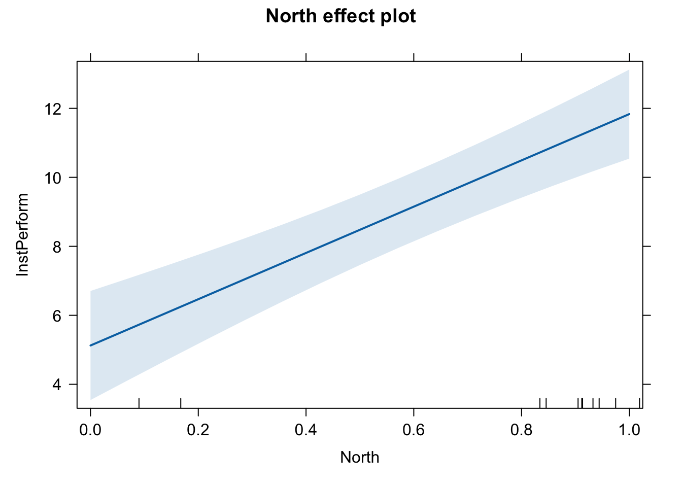
Plot the effect (incorrect version)
plot(effect(term = "North", mod = fit.ns))
library(sjPlot)
##
## Attaching package: 'sjPlot'

## The following object is masked from 'package:ggplot2':
##
##     set_theme
plot_model(fit.ns, type = "pred", terms = c("North"), ci.lvl = 0.95, bpe.style = "line", robust = T, colors = "bw", legend.title = "Elections", vcov.type = c("HC3")) + #,
  theme_bw() +
  ggtitle(element_blank()) +
  labs(x = "North",
       y = "Institutional Performance")
## Warning: `label` cannot be a <ggplot2::element_blank> object.
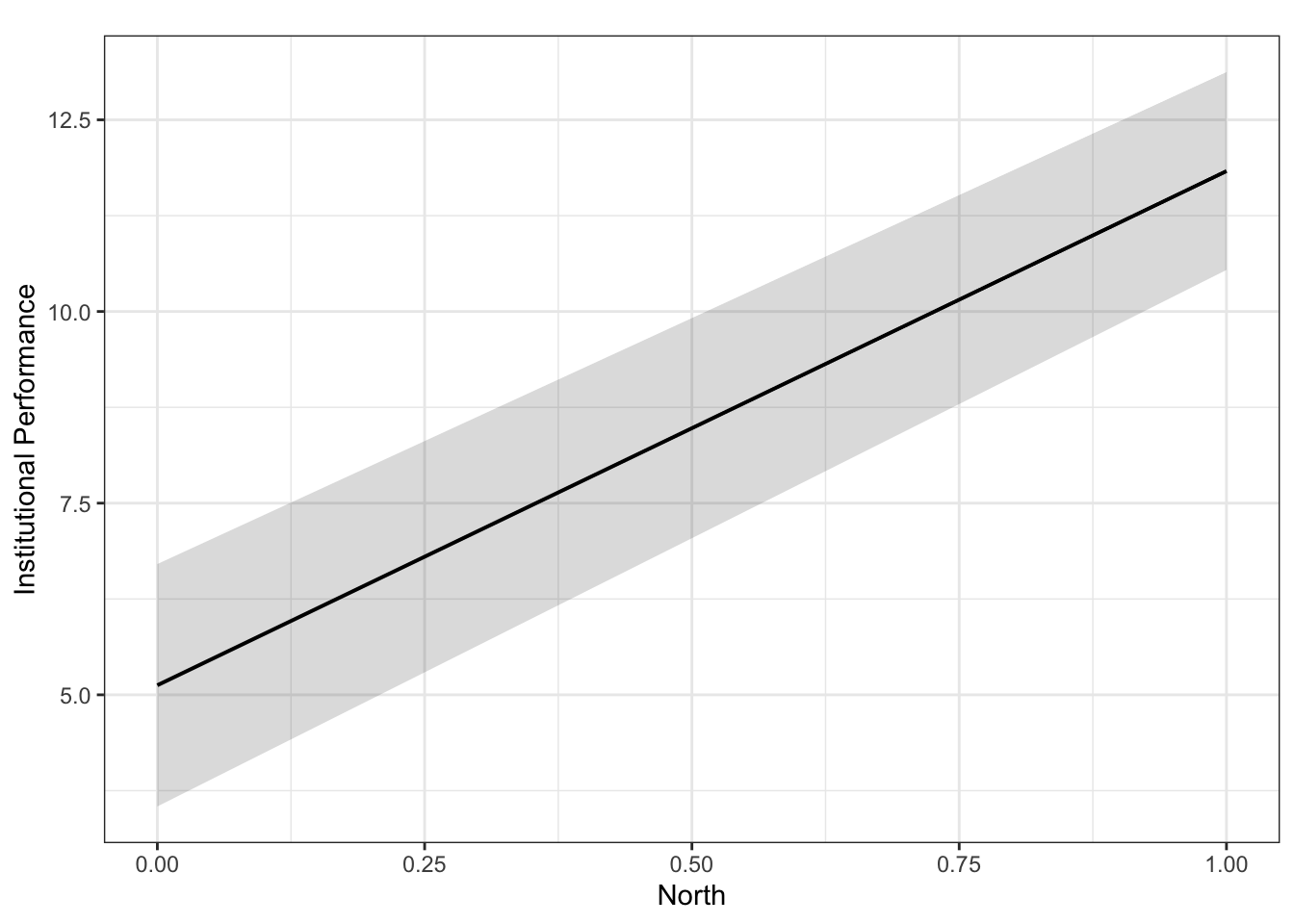
This graph is not ideal for presenting the marginal effect of a dummy variable.
To create a better graph, we need to estimate a model using the original factor variable.
library(tidyverse)
## ── Attaching core tidyverse packages ──────────────────────── tidyverse 2.0.0 ──
## ✔ dplyr     1.1.4     ✔ readr     2.1.5
## ✔ forcats   1.0.0     ✔ stringr   1.5.2
## ✔ lubridate 1.9.3     ✔ tibble    3.3.0
## ✔ purrr     1.1.0     ✔ tidyr     1.3.1
## ── Conflicts ────────────────────────────────────────── tidyverse_conflicts() ──
## ✖ dplyr::filter()     masks stats::filter()
## ✖ dplyr::lag()        masks stats::lag()
## ✖ sjPlot::set_theme() masks ggplot2::set_theme()
## ℹ Use the conflicted package (<http://conflicted.r-lib.org/>) to force all conflicts to become errors
pd $ North = pd $ North %>% as.factor()

fit.ns <- lm(InstPerform ~ North, data = pd)
stargazer(fit.ns, type = "text")
##
## ===============================================
##                         Dependent variable:
##                     ---------------------------
##                             InstPerform
## -----------------------------------------------
## North1                       6.708***
##                               (0.971)
##
## Constant                     5.125***
##                               (0.753)
##
## -----------------------------------------------
## Observations                    20
## R2                             0.726
## Adjusted R2                    0.711
## Residual Std. Error       2.128 (df = 18)
## F Statistic           47.683*** (df = 1; 18)
## ===============================================
## Note:               *p<0.1; **p<0.05; ***p<0.01
plot(effect(term = "North", mod = fit.ns))
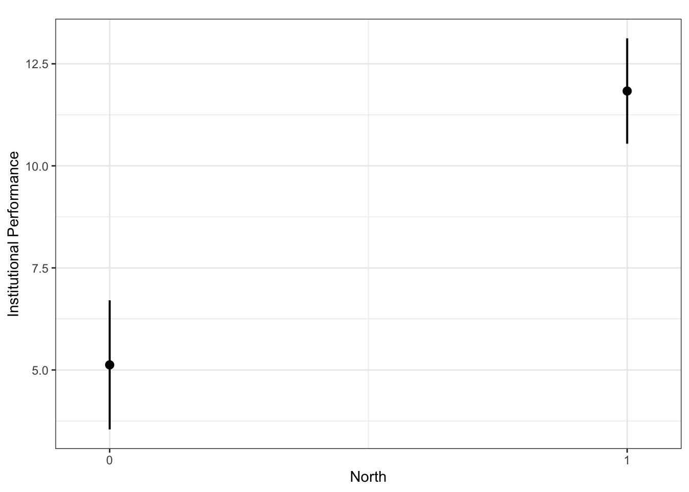
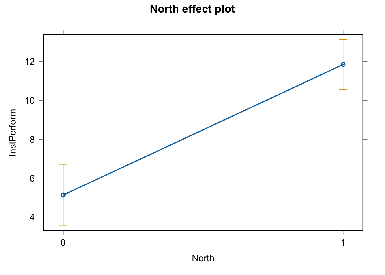 Now we have it.
plot_model(fit.ns, type = "pred", terms = c("North"), ci.lvl = 0.95, bpe.style = "line", robust = T, colors = "bw", legend.title = "Elections", vcov.type = c("HC3")) + #,
  theme_bw() +
  ggtitle(element_blank()) +
  labs(x = "North",
       y = "Institutional Performance")
## Warning: Using `size` aesthetic for lines was deprecated in ggplot2 3.4.0.
## ℹ Please use `linewidth` instead.
## ℹ The deprecated feature was likely used in the ggeffects package.
##   Please report the issue at
##   <https://github.com/strengejacke/ggeffects/issues/>.
## This warning is displayed once every 8 hours.
## Call `lifecycle::last_lifecycle_warnings()` to see where this warning was
## generated.

## Ignoring unknown labels:
## • linetype : "Elections"

## Warning: `label` cannot be a <ggplot2::element_blank> object.
2. Model with no X (constant-only model)
To estimate a model with no X, we put the number 1 in the right-hand-side of the equation, as follows.
fit.nox <- lm(InstPerform ~ 1, data = pd)
stargazer(fit.nox, type = "text")
##
## ===============================================
##                         Dependent variable:
##                     ---------------------------
##                             InstPerform
## -----------------------------------------------
## Constant                     9.150***
##                               (0.885)
##
## -----------------------------------------------
## Observations                    20
## R2                             0.000
## Adjusted R2                    0.000
## Residual Std. Error       3.957 (df = 19)
## ===============================================
## Note:               *p<0.1; **p<0.05; ***p<0.01
The estimated Constant is equal to the mean of Y. This is the “best guess” (best predicted value) of Y when we have no X.
mean( pd $ InstPerform )
## [1] 9.15
R^2 from a constant-only model is always 0, because R^2 measures how much variation in Y is explained by X. Since there is no X, NO variation in Y is explained.
Residual Std. Error (Root Mean Squared Error) from a constant-only model is always equal to the standard deviation of Y, by definition.
sd( pd $ InstPerform )
## [1] 3.957338
3. Model with a non-binary nominal variable (multiple categories without order)
wd <- read.csv("world.csv")

# Suppose we are interested in the effect of region on per capita GDP

# Y (per capita GDP in $ 10,000)
summary(wd $ gdp_10_thou)
##    Min. 1st Qu.  Median    Mean 3rd Qu.    Max.    NA's
##  0.0090  0.0503  0.1897  0.6018  0.6320  4.7354      14
# X (region)
table(wd $ region)
##
##       Africa Asia-Pacific   C&E Europe  Middle East   N. America   S. America
##           49           37           27           19            3           32
##  Scandinavia    W. Europe
##            5           19
head(wd $ region)
## [1] "Middle East" "C&E Europe"  "Africa"      "W. Europe"   "Africa"
## [6] "S. America"
unique(wd $ region)
## [1] "Middle East"  "C&E Europe"   "Africa"       "W. Europe"    "S. America"
## [6] "Asia-Pacific" "N. America"   "Scandinavia"
# This variable has more than one level/factor
Regression with one nominal variable (factor)
One way to analyze the relationship between Y and a non-binary nominal variable is to estimate a regression of Y on the original factor variable (i.e., include the original factor variable as is).
fit.gr <- lm(gdp_10_thou ~ region, data = wd)

stargazer(fit.gr, type = "text")
##
## ===============================================
##                         Dependent variable:
##                     ---------------------------
##                             gdp_10_thou
## -----------------------------------------------
## regionAsia-Pacific            0.332**
##                               (0.131)
##
## regionC&E Europe               0.178
##                               (0.137)
##
## regionMiddle East            0.668***
##                               (0.161)
##
## regionN. America             2.077***
##                               (0.339)
##
## regionS. America              0.284**
##                               (0.131)
##
## regionScandinavia            3.030***
##                               (0.267)
##
## regionW. Europe              2.230***
##                               (0.168)
##
## Constant                       0.093
##                               (0.082)
##
## -----------------------------------------------
## Observations                    177
## R2                             0.651
## Adjusted R2                    0.636
## Residual Std. Error      0.569 (df = 169)
## F Statistic           45.006*** (df = 7; 169)
## ===============================================
## Note:               *p<0.1; **p<0.05; ***p<0.01
R will internally create 8 dummy variables and include 7 of them, dropping the first dummy variable (regionAfrica).
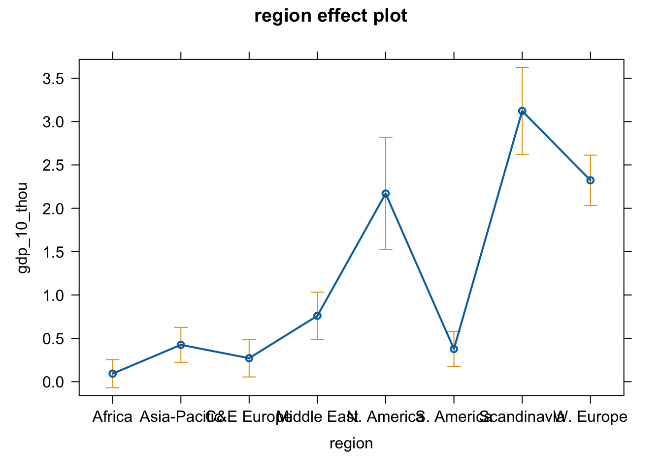
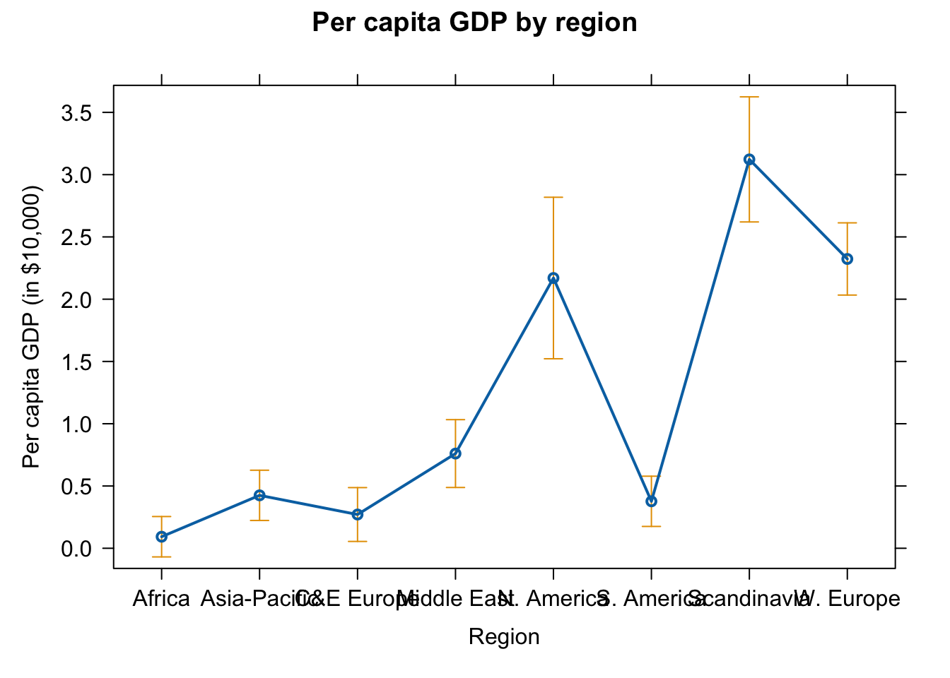
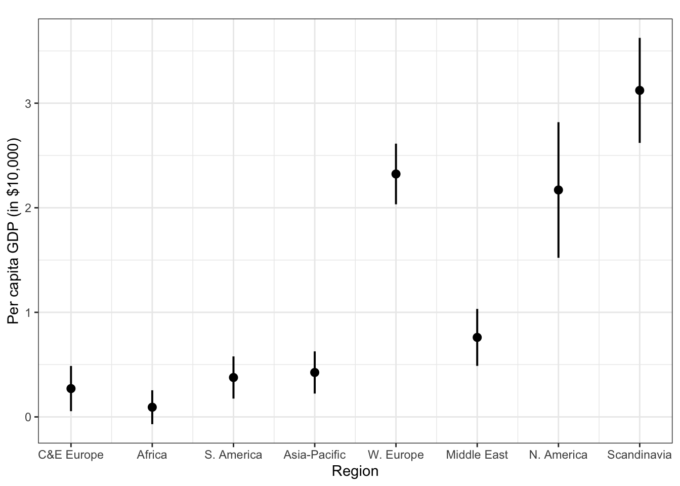
Plot the effect of region
plot(effect(term = "region", mod = fit.gr))
# Change the axis labels and graph title
# pdf(file = "Region_me.pdf", width = 8, height = 5)
plot(effect(term = "region", mod = fit.gr),
     main = "Per capita GDP by region",
     xlab = "Region", ylab = "Per capita GDP (in $10,000)")
# dev.off()
plot_model(fit.gr, type = "pred", terms = c("region"), ci.lvl = 0.95, bpe.style = "line", robust = T, colors = "bw", legend.title = "Elections", vcov.type = c("HC3")) + #,
  theme_bw() +
  ggtitle(element_blank()) +
  labs(x = "Region",
       y = "Per capita GDP (in $10,000)")
## Ignoring unknown labels:
## • linetype : "Elections"

## Warning: `label` cannot be a <ggplot2::element_blank> object.
Manually create k dummy variables
Alternatively, we can manually create k dummy variables ourselves and include them in a regression.
Let’s first create a series of dummy variables
wd $ Africa <- ifelse(wd $ region == "Africa", 1, 0)
wd $ AsiaPacific <- ifelse(wd $ region == "Asia-Pacific", 1, 0)
wd $ CEEurope <- ifelse(wd $ region == "C&E Europe", 1, 0)
wd $ MiddleEast <- ifelse(wd $ region == "Middle East", 1, 0)
wd $ NAmerica <- ifelse(wd $ region == "N. America", 1, 0)
wd $ SAmerica <- ifelse(wd $ region == "S. America", 1, 0)
wd $ Scandinavia <- ifelse(wd $ region == "Scandinavia", 1, 0)
wd $ WEurope <- ifelse(wd $ region == "W. Europe", 1, 0)


wd[1:10, c("region", "Africa", "AsiaPacific", "CEEurope", "MiddleEast", "NAmerica","SAmerica","Scandinavia","WEurope")]
##          region Africa AsiaPacific CEEurope MiddleEast NAmerica SAmerica
## 1   Middle East      0           0        0          1        0        0
## 2    C&E Europe      0           0        1          0        0        0
## 3        Africa      1           0        0          0        0        0
## 4     W. Europe      0           0        0          0        0        0
## 5        Africa      1           0        0          0        0        0
## 6    S. America      0           0        0          0        0        1
## 7    S. America      0           0        0          0        0        1
## 8    C&E Europe      0           0        1          0        0        0
## 9  Asia-Pacific      0           1        0          0        0        0
## 10    W. Europe      0           0        0          0        0        0
##    Scandinavia WEurope
## 1            0       0
## 2            0       0
## 3            0       0
## 4            0       1
## 5            0       0
## 6            0       0
## 7            0       0
## 8            0       0
## 9            0       0
## 10           0       1
For the first row, region is equal to Middle East and so only the Middle East dummy takes the value of 1 and all the other dummy variables are coded as 0. Likewise, for the second observation, only the CEEurope dummy is 1 and everything else is 0.
Since there are 8 categories, we actually need only 7 dummy variables to completely describe the values of the region variable. In running a regression model, we thus need to include 7 of the 8 dummy variables. The omitted category will be used as the baseline.
Let’s now estimate a regression model where 7 dummy variables are included in the RHS. We will drop the Africa dummy.
fit.gr.1 <- lm(gdp_10_thou ~
                 # Africa +
                 AsiaPacific +
                 CEEurope +
                 MiddleEast +
                 NAmerica +
                 SAmerica +
                 Scandinavia +
                 WEurope,
               data = wd )

stargazer(fit.gr.1, type = "text")
##
## ===============================================
##                         Dependent variable:
##                     ---------------------------
##                             gdp_10_thou
## -----------------------------------------------
## AsiaPacific                   0.332**
##                               (0.131)
##
## CEEurope                       0.178
##                               (0.137)
##
## MiddleEast                   0.668***
##                               (0.161)
##
## NAmerica                     2.077***
##                               (0.339)
##
## SAmerica                      0.284**
##                               (0.131)
##
## Scandinavia                  3.030***
##                               (0.267)
##
## WEurope                      2.230***
##                               (0.168)
##
## Constant                       0.093
##                               (0.082)
##
## -----------------------------------------------
## Observations                    177
## R2                             0.651
## Adjusted R2                    0.636
## Residual Std. Error      0.569 (df = 169)
## F Statistic           45.006*** (df = 7; 169)
## ===============================================
## Note:               *p<0.1; **p<0.05; ***p<0.01
The results are exactly the same as the one we obtained before.
stargazer(fit.gr, fit.gr.1, type = "text")
##
## ===========================================================
##                                    Dependent variable:
##                                ----------------------------
##                                        gdp_10_thou
##                                     (1)            (2)
## -----------------------------------------------------------
## regionAsia-Pacific                0.332**
##                                   (0.131)
##
## regionC&E Europe                   0.178
##                                   (0.137)
##
## regionMiddle East                 0.668***
##                                   (0.161)
##
## regionN. America                  2.077***
##                                   (0.339)
##
## regionS. America                  0.284**
##                                   (0.131)
##
## regionScandinavia                 3.030***
##                                   (0.267)
##
## regionW. Europe                   2.230***
##                                   (0.168)
##
## AsiaPacific                                      0.332**
##                                                  (0.131)
##
## CEEurope                                          0.178
##                                                  (0.137)
##
## MiddleEast                                      0.668***
##                                                  (0.161)
##
## NAmerica                                        2.077***
##                                                  (0.339)
##
## SAmerica                                         0.284**
##                                                  (0.131)
##
## Scandinavia                                     3.030***
##                                                  (0.267)
##
## WEurope                                         2.230***
##                                                  (0.168)
##
## Constant                           0.093          0.093
##                                   (0.082)        (0.082)
##
## -----------------------------------------------------------
## Observations                        177            177
## R2                                 0.651          0.651
## Adjusted R2                        0.636          0.636
## Residual Std. Error (df = 169)     0.569          0.569
## F Statistic (df = 7; 169)        45.006***      45.006***
## ===========================================================
## Note:                           *p<0.1; **p<0.05; ***p<0.01
In both of the models, the Africa dummy is excluded, so Africa is used as the baseline. This means that the estimated Constant represents the predicted value of Y for Africa, because this is the predicted value of Y when ALL the independent variables are equal to 0.
To obtain the predicted value of Y for other regions, we can simply add Constant (0.093) to the estimated coefficient for the corresponding region. For example, the predicted Y for NAmerica is 0.093 + 2.077 = 2.17.
An even better way to obtain the same results is to estimate a model that includes all 8 dummies but drops the constant. To drop a constant, we add “+ 0” in the right-hand-side of the equation, as follows.
fit.gr.2 <- lm(gdp_10_thou ~
                 Africa +
                 AsiaPacific +
                 CEEurope +
                 MiddleEast +
                 NAmerica +
                 SAmerica +
                 Scandinavia +
                 WEurope + 0,
               data = wd )

stargazer(fit.gr.2, type = "text")
##
## ===============================================
##                         Dependent variable:
##                     ---------------------------
##                             gdp_10_thou
## -----------------------------------------------
## Africa                         0.093
##                               (0.082)
##
## AsiaPacific                  0.425***
##                               (0.102)
##
## CEEurope                      0.271**
##                               (0.109)
##
## MiddleEast                   0.760***
##                               (0.138)
##
## NAmerica                     2.170***
##                               (0.328)
##
## SAmerica                     0.377***
##                               (0.102)
##
## Scandinavia                  3.123***
##                               (0.254)
##
## WEurope                      2.323***
##                               (0.147)
##
## -----------------------------------------------
## Observations                    177
## R2                             0.752
## Adjusted R2                    0.741
## Residual Std. Error      0.569 (df = 169)
## F Statistic           64.143*** (df = 8; 169)
## ===============================================
## Note:               *p<0.1; **p<0.05; ***p<0.01
Let’s compare the two results to see that these two models are mathematically equivalent.
stargazer(fit.gr.1, fit.gr.2, type = "text")
##
## ==============================================================================
##                                              Dependent variable:
##                                -----------------------------------------------
##                                                  gdp_10_thou
##                                          (1)                     (2)
## ------------------------------------------------------------------------------
## Africa                                                          0.093
##                                                                (0.082)
##
## AsiaPacific                            0.332**                0.425***
##                                        (0.131)                 (0.102)
##
## CEEurope                                0.178                  0.271**
##                                        (0.137)                 (0.109)
##
## MiddleEast                            0.668***                0.760***
##                                        (0.161)                 (0.138)
##
## NAmerica                              2.077***                2.170***
##                                        (0.339)                 (0.328)
##
## SAmerica                               0.284**                0.377***
##                                        (0.131)                 (0.102)
##
## Scandinavia                           3.030***                3.123***
##                                        (0.267)                 (0.254)
##
## WEurope                               2.230***                2.323***
##                                        (0.168)                 (0.147)
##
## Constant                                0.093
##                                        (0.082)
##
## ------------------------------------------------------------------------------
## Observations                             177                     177
## R2                                      0.651                   0.752
## Adjusted R2                             0.636                   0.741
## Residual Std. Error (df = 169)          0.569                   0.569
## F Statistic                    45.006*** (df = 7; 169) 64.143*** (df = 8; 169)
## ==============================================================================
## Note:                                              *p<0.1; **p<0.05; ***p<0.01
Even though the estimated coefficients are slightly different, they really are the same model. To see how, try calculating the predicted value of Y for NAmerica with model (1) and with model (2).
If we use the first model, the predicted value of Y for N. America is 0.093 (which is the intercept) + 2.077 (which is the slope for NAmerica) as we saw above. It is equal to 0.093 + 2.077 = 2.17.
On the other hand, if we use the second model, the predicted value of Y for N. America is simply 2.170 (slope for NAmerica).
So both models say that it’s 2.17. This is not a coincidence. We would obtain the same predicted values for other regions as well. This is because, again, the two models are equivalent. These two are simply using two different ways to express the same pattern.
Notice that Residual Std. Error from both models are exactly the same.
However, R^2 from these models are different. This is because one model has a Constant and the other model doesn’t.
What would happen if we fail to drop one dummy variable NOR drop the intercept…?
fit.gr.n <- lm(gdp_10_thou ~  Africa + AsiaPacific + CEEurope + MiddleEast +
                 NAmerica + SAmerica + Scandinavia + WEurope, data = wd )

stargazer(fit.gr.n, type = "text")
##
## ===============================================
##                         Dependent variable:
##                     ---------------------------
##                             gdp_10_thou
## -----------------------------------------------
## Africa                       -2.230***
##                               (0.168)
##
## AsiaPacific                  -1.898***
##                               (0.179)
##
## CEEurope                     -2.052***
##                               (0.183)
##
## MiddleEast                   -1.563***
##                               (0.202)
##
## NAmerica                      -0.153
##                               (0.360)
##
## SAmerica                     -1.946***
##                               (0.179)
##
## Scandinavia                  0.799***
##                               (0.294)
##
## WEurope
##
##
## Constant                     2.323***
##                               (0.147)
##
## -----------------------------------------------
## Observations                    177
## R2                             0.651
## Adjusted R2                    0.636
## Residual Std. Error      0.569 (df = 169)
## F Statistic           45.006*** (df = 7; 169)
## ===============================================
## Note:               *p<0.1; **p<0.05; ***p<0.01
What happens is that R will just simply drop the LAST dummy variable (WEurope) automatically. This is not wrong, but it is not ideal, either. As I mentioned above, the best approach here is to include ALL dummy variables and drop the constant.
4. Model with an ordinal X (multiple categories with order)
# Y: Government effectiveness
summary(wd $ effectiveness)
##    Min. 1st Qu.  Median    Mean 3rd Qu.    Max.    NA's
##    0.00   28.19   40.31   45.77   62.77  100.00       5
# X: Ethnic fractionalization level
table(wd $ frac_eth3)
##
##          High    Low Medium
##      3     62     62     64
Note 1: Notice that the frequency table above has a mysterious blank column (with 3 observations). This indicates that there are 3 observations that are not categorized as any of the three values (High, Medium, or Low).
In other words, the value of this variable is missing for these 3 observations,but they are not properly coded as NA. This can cause a big problem in running a regression, so let’s fix this.
We fix this by recoding these 3 observations as NA.
wd $ frac_eth3[wd $ frac_eth3 == ""] <- NA

table(wd $ frac_eth3)
##
##   High    Low Medium
##     62     62     64
# We still have a blank column, but there is 0 observation now.
Automatic approach 1 (let R handle the issue)
The frac_eth3 is an ordinal variable. Ordinal variables are also categorical variables, and so they are stored as a factor variable in R.
As we saw above, there are automatic and manual approaches when it comes to handling factor variables in regression.
Let’s first see the automatic approach.
fit.ge.0 <- lm(effectiveness ~ frac_eth3, data = wd)
stargazer(fit.ge.0, type = "text")
##
## ===============================================
##                         Dependent variable:
##                     ---------------------------
##                            effectiveness
## -----------------------------------------------
## frac_eth3Low                 20.443***
##                               (4.000)
##
## frac_eth3Medium              13.347***
##                               (4.000)
##
## Constant                     34.736***
##                               (2.828)
##
## -----------------------------------------------
## Observations                    183
## R2                             0.130
## Adjusted R2                    0.120
## Residual Std. Error      22.090 (df = 180)
## F Statistic           13.468*** (df = 2; 180)
## ===============================================
## Note:               *p<0.1; **p<0.05; ***p<0.01
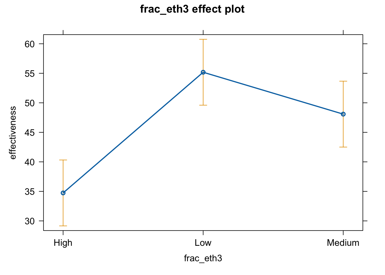
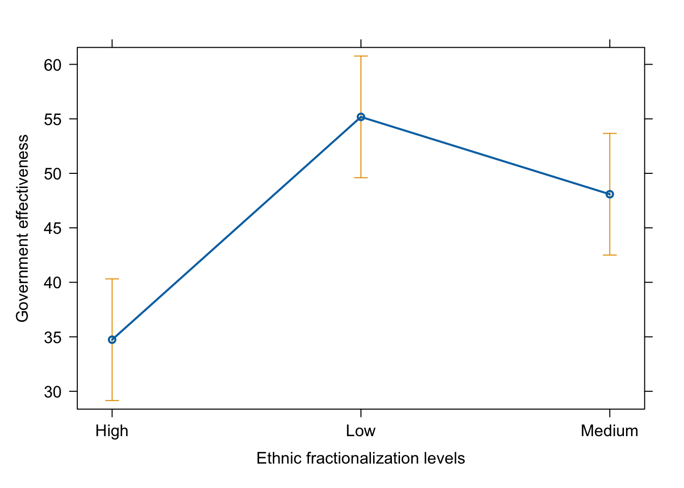
As we saw in the lecture, the results are not really intuitive. R stores this variable as a factor variable, but it doesn’t recognize that there is a natural order in the values (Low –> High) or (High –> Low). R simply orders the three values (High, Medium, Low) alphabetically.
We will fix this later, but let’s first see what the effect graph would look like if we simply adopt the automatic approach.
plot(effect(term = "frac_eth3", mod = fit.ge.0))
# pdf(file = "frac3_me_auto1.pdf", width = 8, height = 5)
plot(effect(term = "frac_eth3", mod = fit.ge.0),
  main = "",
  xlab = "Ethnic fractionalization levels",
  ylab = "Government effectiveness")
# dev.off()
Automatic approach 2 (fix the ordering first)
We will now fix the ordering of the frac_eth3 variable.
wd $ frac_eth3_ord <- factor(wd $ frac_eth3,
  levels = c("Low", "Medium", "High"))
In writing down the values for the levels option, arrange them in the “natural” order (either Low to High or High to Low).
Whenever we create a new variable by recoding an existing one, we should check if it worked correctly.
table(wd $ frac_eth3)
##
##   High    Low Medium
##     62     62     64
table(wd $ frac_eth3_ord)
##
##    Low Medium   High
##     62     64     62
table(wd $ frac_eth3_ord, wd $ frac_eth3)
##
##          High Low Medium
##   Low       0  62      0
##   Medium    0   0     64
##   High     62   0      0
Now let’s estimate a regression with this variable
fit.ge.1 <- lm(effectiveness ~ frac_eth3_ord, data = wd)
stargazer(fit.ge.1, type = "text")
##
## ===============================================
##                         Dependent variable:
##                     ---------------------------
##                            effectiveness
## -----------------------------------------------
## frac_eth3_ordMedium           -7.096*
##                               (4.000)
##
## frac_eth3_ordHigh           -20.443***
##                               (4.000)
##
## Constant                     55.180***
##                               (2.828)
##
## -----------------------------------------------
## Observations                    183
## R2                             0.130
## Adjusted R2                    0.120
## Residual Std. Error      22.090 (df = 180)
## F Statistic           13.468*** (df = 2; 180)
## ===============================================
## Note:               *p<0.1; **p<0.05; ***p<0.01
Compare the two models (automatic 1 and automatic 2)
stargazer(fit.ge.0, fit.ge.1, type = "text")
##
## ===========================================================
##                                    Dependent variable:
##                                ----------------------------
##                                       effectiveness
##                                     (1)            (2)
## -----------------------------------------------------------
## frac_eth3Low                     20.443***
##                                   (4.000)
##
## frac_eth3Medium                  13.347***
##                                   (4.000)
##
## frac_eth3_ordMedium                              -7.096*
##                                                  (4.000)
##
## frac_eth3_ordHigh                              -20.443***
##                                                  (4.000)
##
## Constant                         34.736***      55.180***
##                                   (2.828)        (2.828)
##
## -----------------------------------------------------------
## Observations                        183            183
## R2                                 0.130          0.130
## Adjusted R2                        0.120          0.120
## Residual Std. Error (df = 180)     22.090        22.090
## F Statistic (df = 2; 180)        13.468***      13.468***
## ===========================================================
## Note:                           *p<0.1; **p<0.05; ***p<0.01
# Notice that the two models are equivalent, despite the difference in appearances.

# The two are equivalent in the sense that
#  (a) model fit statistics are the same;
#  (b) predicted values for Low, Medium, High are the same.

# We can easily see (a) by looking at the table.
# You can convince yourself about (b) by calculating the predicted values
# for Low, Medium, and High.

# From model (1)
#   High:   34.736
#   Low:    34.736 + 20.443 = 55.179
#   Medium: 34.736 + 13.347 = 48.083

# From model (2)
#   Low:    55.180
#   Medium: 55.180 - 7.096 = 48.084
#   High:   55.180 - 20.443 = 34.737
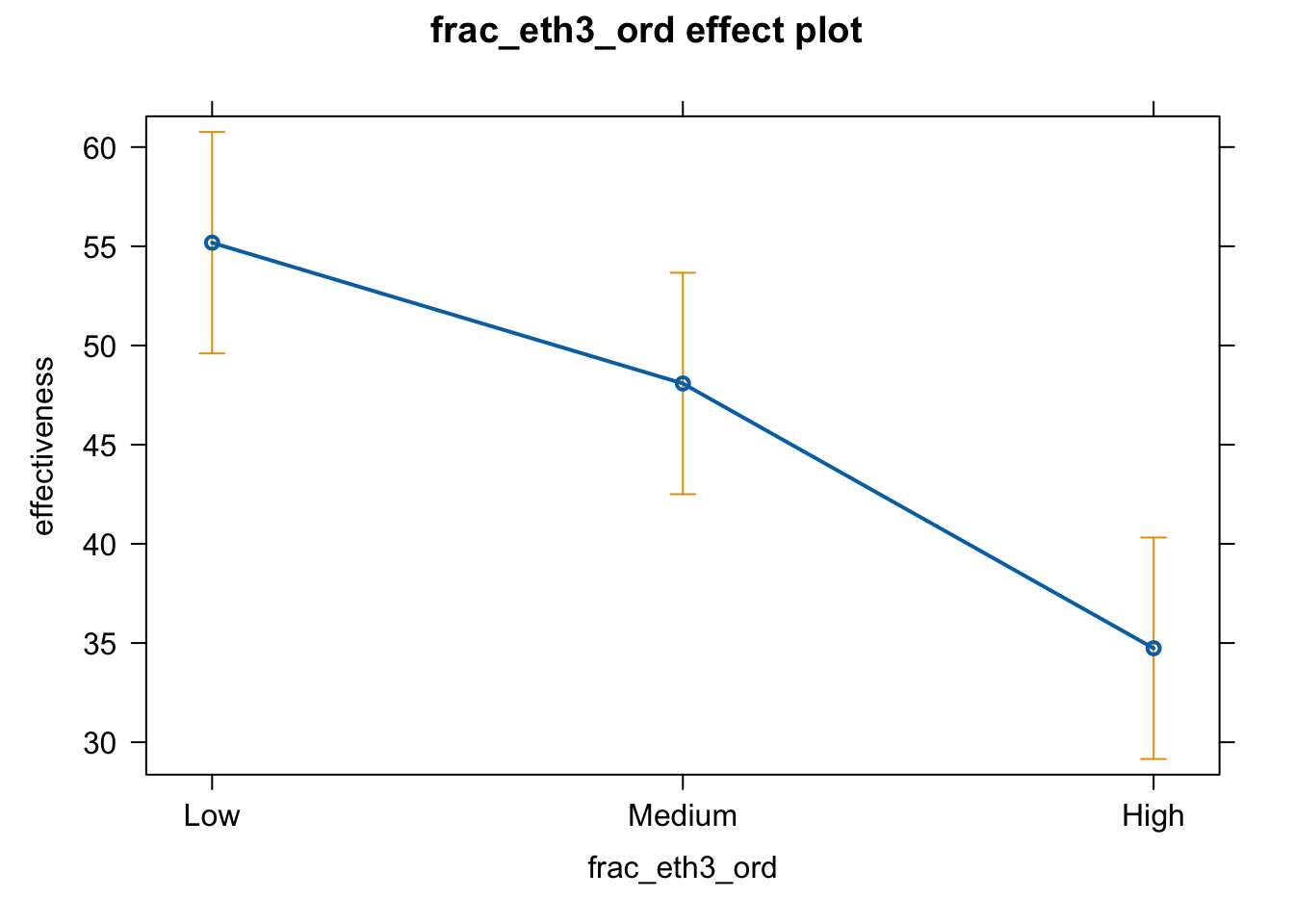
Except for differences due to rounding, the two sets of three predicted are identical.
These two models are just different representations of the same relationship.
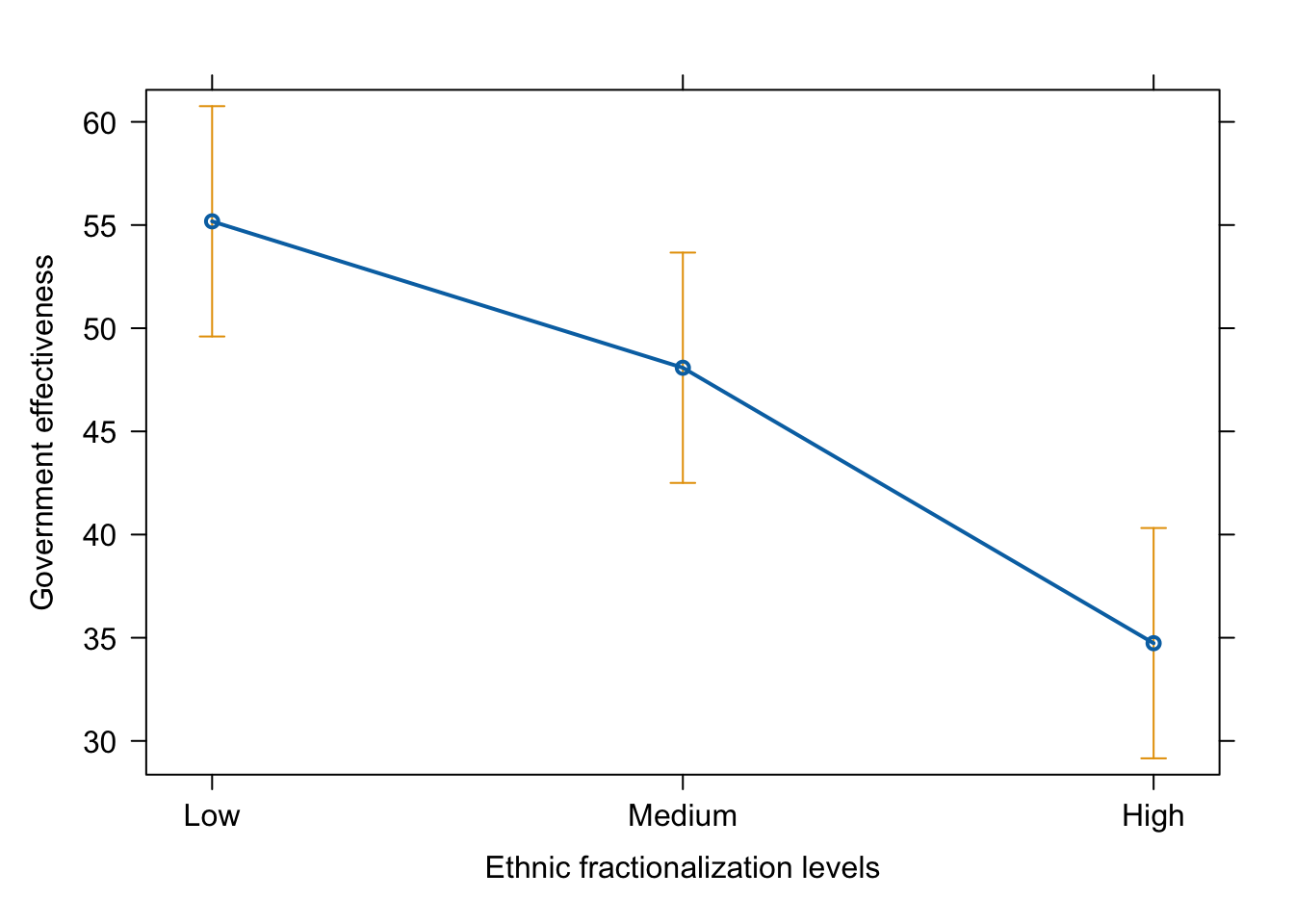
Effect plot
plot(effect(term = "frac_eth3_ord", mod = fit.ge.1))
# pdf(file = "frac3_me_auto2.pdf", width = 8, height = 5)
plot(effect(term = "frac_eth3_ord", mod = fit.ge.1),
  main = "",
  xlab = "Ethnic fractionalization levels",
  ylab = "Government effectiveness")
# dev.off()
Manual approach
Let’s now apply the manual approach.
We create a series of dummy variables first
wd $ frac_eth3_Low <- ifelse(wd $ frac_eth3 == "Low", 1, 0)
wd $ frac_eth3_Medium <- ifelse(wd $ frac_eth3 == "Medium", 1, 0)
wd $ frac_eth3_High <- ifelse(wd $ frac_eth3 == "High", 1, 0)

# and include all of them AND drop the constant

fit.ge.2 <- lm(effectiveness ~ frac_eth3_Low + frac_eth3_Medium +
    frac_eth3_High + 0,
  data = wd)

stargazer(fit.ge.2, type = "text")
##
## ===============================================
##                         Dependent variable:
##                     ---------------------------
##                            effectiveness
## -----------------------------------------------
## frac_eth3_Low                55.180***
##                               (2.828)
##
## frac_eth3_Medium             48.084***
##                               (2.828)
##
## frac_eth3_High               34.736***
##                               (2.828)
##
## -----------------------------------------------
## Observations                    183
## R2                             0.820
## Adjusted R2                    0.817
## Residual Std. Error      22.090 (df = 180)
## F Statistic          273.482*** (df = 3; 180)
## ===============================================
## Note:               *p<0.1; **p<0.05; ***p<0.01
We can see that ethnic fractionalization level has a negative effect on government effectiveness.
Compare the tables from automatic and manual approaches.
stargazer(fit.ge.0, fit.ge.2, type = "text", omit.stat = "f")
##
## ===========================================================
##                                    Dependent variable:
##                                ----------------------------
##                                       effectiveness
##                                     (1)            (2)
## -----------------------------------------------------------
## frac_eth3Low                     20.443***
##                                   (4.000)
##
## frac_eth3Medium                  13.347***
##                                   (4.000)
##
## frac_eth3_Low                                   55.180***
##                                                  (2.828)
##
## frac_eth3_Medium                                48.084***
##                                                  (2.828)
##
## frac_eth3_High                                  34.736***
##                                                  (2.828)
##
## Constant                         34.736***
##                                   (2.828)
##
## -----------------------------------------------------------
## Observations                        183            183
## R2                                 0.130          0.820
## Adjusted R2                        0.120          0.817
## Residual Std. Error (df = 180)     22.090        22.090
## ===========================================================
## Note:                           *p<0.1; **p<0.05; ***p<0.01
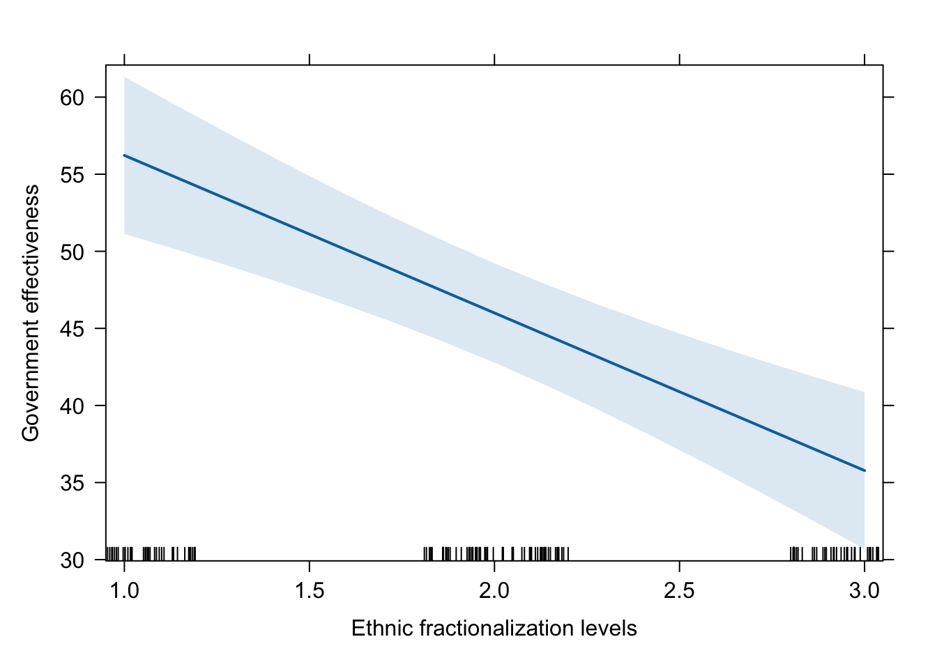
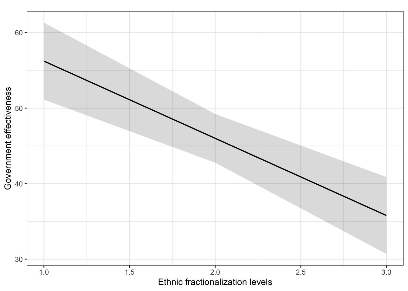
Third approach: treat it as numerical
First, we need to convert the ordinal frac_eth3_ord into numeric
wd $ num.frac_eth3 <- as.numeric(wd $ frac_eth3_ord)

table(wd $ num.frac_eth3, wd $ frac_eth3_ord)
##
##     Low Medium High
##   1  62      0    0
##   2   0     64    0
##   3   0      0   62
We can see that “Low” is now changed into 1, “Medium” is 2, and “High” is 3.
It is really important that we use here the ORDERED version of frac_eth3 that we manually created above, not the original frac_eth3. Recall that the original frac_eth3 has the “wrong” ordering: High, Low, Medium.
fit.ge.3 <- lm(effectiveness ~ num.frac_eth3, data = wd)

stargazer(fit.ge.3, type = "text")
##
## ===============================================
##                         Dependent variable:
##                     ---------------------------
##                            effectiveness
## -----------------------------------------------
## num.frac_eth3               -10.222***
##                               (1.999)
##
## Constant                     66.443***
##                               (4.318)
##
## -----------------------------------------------
## Observations                    183
## R2                             0.126
## Adjusted R2                    0.121
## Residual Std. Error      22.079 (df = 181)
## F Statistic           26.148*** (df = 1; 181)
## ===============================================
## Note:               *p<0.1; **p<0.05; ***p<0.01
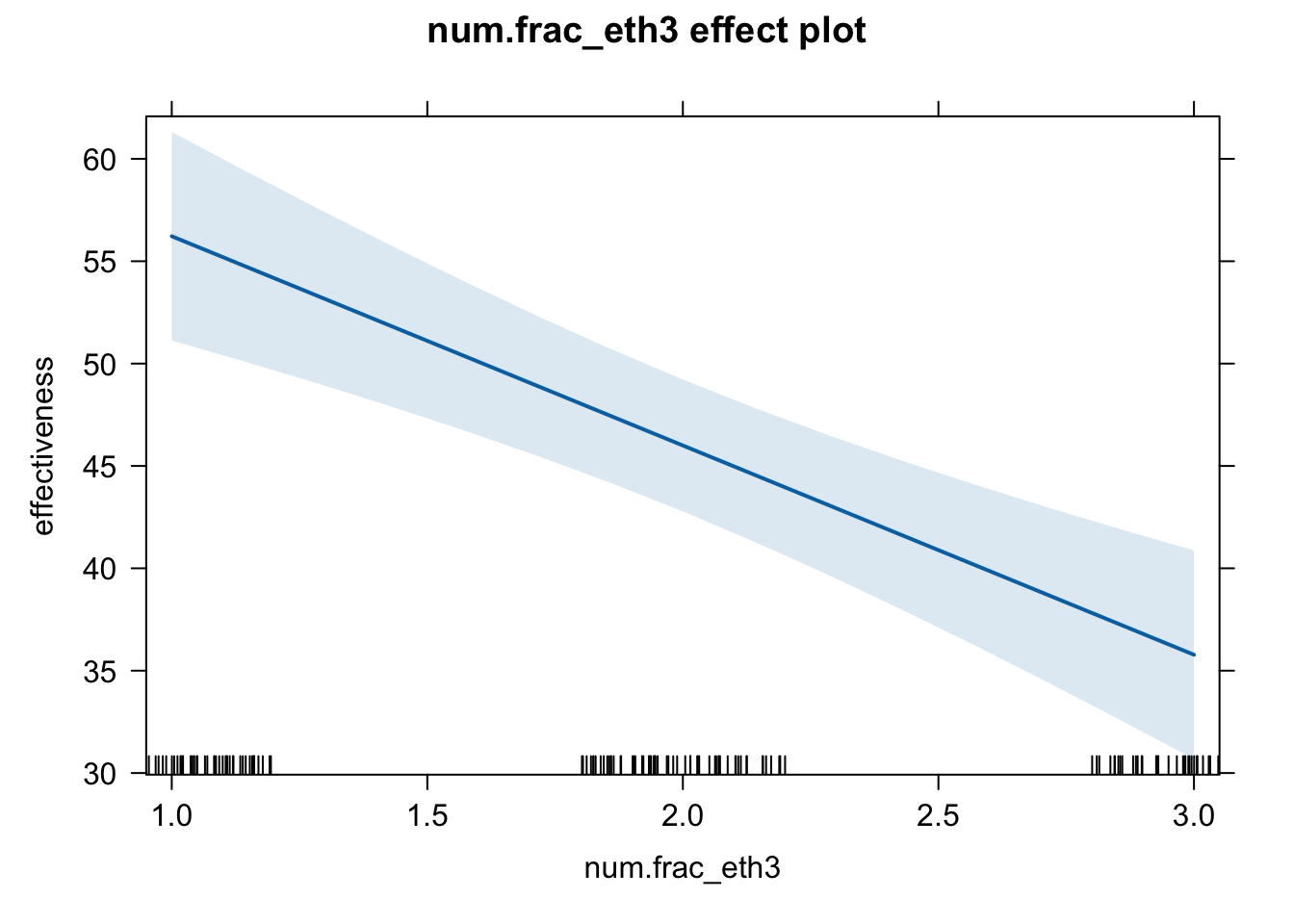
plot(effect(term = "num.frac_eth3", mod = fit.ge.3))
# pdf(file = "frac_num_me.pdf", width = 8, height = 5)
plot(effect(term = "num.frac_eth3", mod = fit.ge.3),
  main = "",
  xlab = "Ethnic fractionalization levels",
  ylab = "Government effectiveness")
# dev.off()
plot_model(fit.ge.3, type = "pred", terms = c("num.frac_eth3"), ci.lvl = 0.95, bpe.style = "line", robust = T, colors = "bw", legend.title = "Elections", vcov.type = c("HC3")) + #,
  theme_bw() +
  ggtitle(element_blank()) +
  labs(x = "Ethnic fractionalization levels",
       y = "Government effectiveness")
## Warning: `label` cannot be a <ggplot2::element_blank> object.
Compare the Method 1 and Method 2 results
stargazer(fit.ge.2, fit.ge.3, type = "text", omit.stat = "f")
##
## =======================================================
##                             Dependent variable:
##                     -----------------------------------
##                                effectiveness
##                            (1)               (2)
## -------------------------------------------------------
## frac_eth3_Low           55.180***
##                          (2.828)
##
## frac_eth3_Medium        48.084***
##                          (2.828)
##
## frac_eth3_High          34.736***
##                          (2.828)
##
## num.frac_eth3                            -10.222***
##                                            (1.999)
##
## Constant                                  66.443***
##                                            (4.318)
##
## -------------------------------------------------------
## Observations               183               183
## R2                        0.820             0.126
## Adjusted R2               0.817             0.121
## Residual Std. Error 22.090 (df = 180) 22.079 (df = 181)
## =======================================================
## Note:                       *p<0.1; **p<0.05; ***p<0.01
Here, the two models are NOT mathematically equivalent. The first model (dummy approach) is more flexible. If the more flexible model fits the data better (has a smaller RMSE), you should choose the more flexible model as the best model.
However, it may be OK to choose the less flexible model (i.e., the numeric approach) when one or more of the following conditions hold:
- RMSE for the less flexible model is not much smaller compared with the more flexible one;
- Your ordinal variable has too many (more than 5) categories;
- The ordinal variable is NOT your main independent variable (i.e., it’s just a control variable).
In our current example, RMSE is actually smaller for the less flexible model. Also, the flexible model suggests that the relationship is almost linear, as we saw in the plot (second plot on Slide 50). So, it is OK to use the numeric one, if frac_eth3 is just a control variable (i.e., not your main independent variable).