Interaction model
Data (Japanese election data) for this lab can be found here
# Preparation -------------------------------------------------------------
rm(list = ls())       # delete everything in the memory
library(foreign)      # for read.dta
library(ggplot2)      # for graphics
library(stargazer)    # Regression table
library(effects)
Numerical × binary interaction
Example: Japanese election data
## Japanese election data
je <- read.dta("/Users/howardliu/methodsPol/content/class/jelec2009.dta")
The unit of observation is an individual candidate who ran in the 2009 general election in Japan.
The variables of our primary interests are:
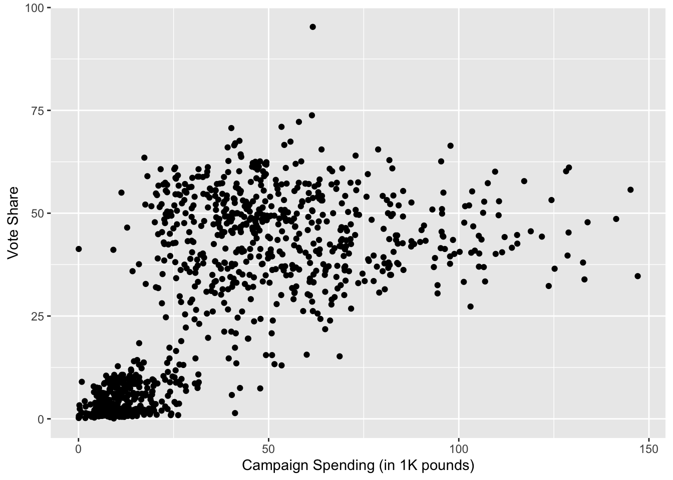
Y: voteshare % of votes a candidate received in his/her electoral district
X: exp amount of money (measured in 1000 pounds) the candidate spent on his/her campaign.
# scatterplot
g <- ggplot(je, aes(x = exp, y = voteshare)) + geom_point()
g <- g + ylab("Vote Share") + xlab("Campaign Spending (in 1K pounds)")
g
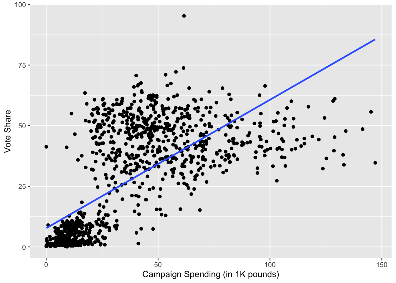
# scatterplot with the fitted line
g <- ggplot(je, aes(x = exp, y = voteshare)) + geom_point()
g <- g + ylab("Vote Share") + xlab("Campaign Spending (in 1K pounds)")
g <- g + geom_smooth(method = lm, alpha = 0)
g
## `geom_smooth()` using formula = 'y ~ x'
# simple linear regression (ignoring a third variable)
fit.1 <- lm(voteshare ~ exp, data = je)
stargazer(fit.1, type = "text")
##
## ===============================================
##                         Dependent variable:
##                     ---------------------------
##                              voteshare
## -----------------------------------------------
## exp                          0.530***
##                               (0.017)
##
## Constant                     7.735***
##                               (0.757)
##
## -----------------------------------------------
## Observations                   1,124
## R2                             0.478
## Adjusted R2                    0.478
## Residual Std. Error     16.042 (df = 1122)
## F Statistic         1,028.236*** (df = 1; 1122)
## ===============================================
## Note:               *p<0.1; **p<0.05; ***p<0.01
Controlling for incumbency status (additive model)
Let’s say we suspect that incumbency status (incumbent or challenger) might influence both X and Y positively, and so a failure to control for this would generate a positive omitted variable bias in our assessment of the relationship between exp (campaign spending) and voteshare.
Take a look at the incumbency variable (Z)
table(je $ incumbent)
##
## non-incumbent     incumbent
##           732           392
note that the variable “incumbent” takes the value of 0 for “non-incumbent” and 1 for “incumbent”
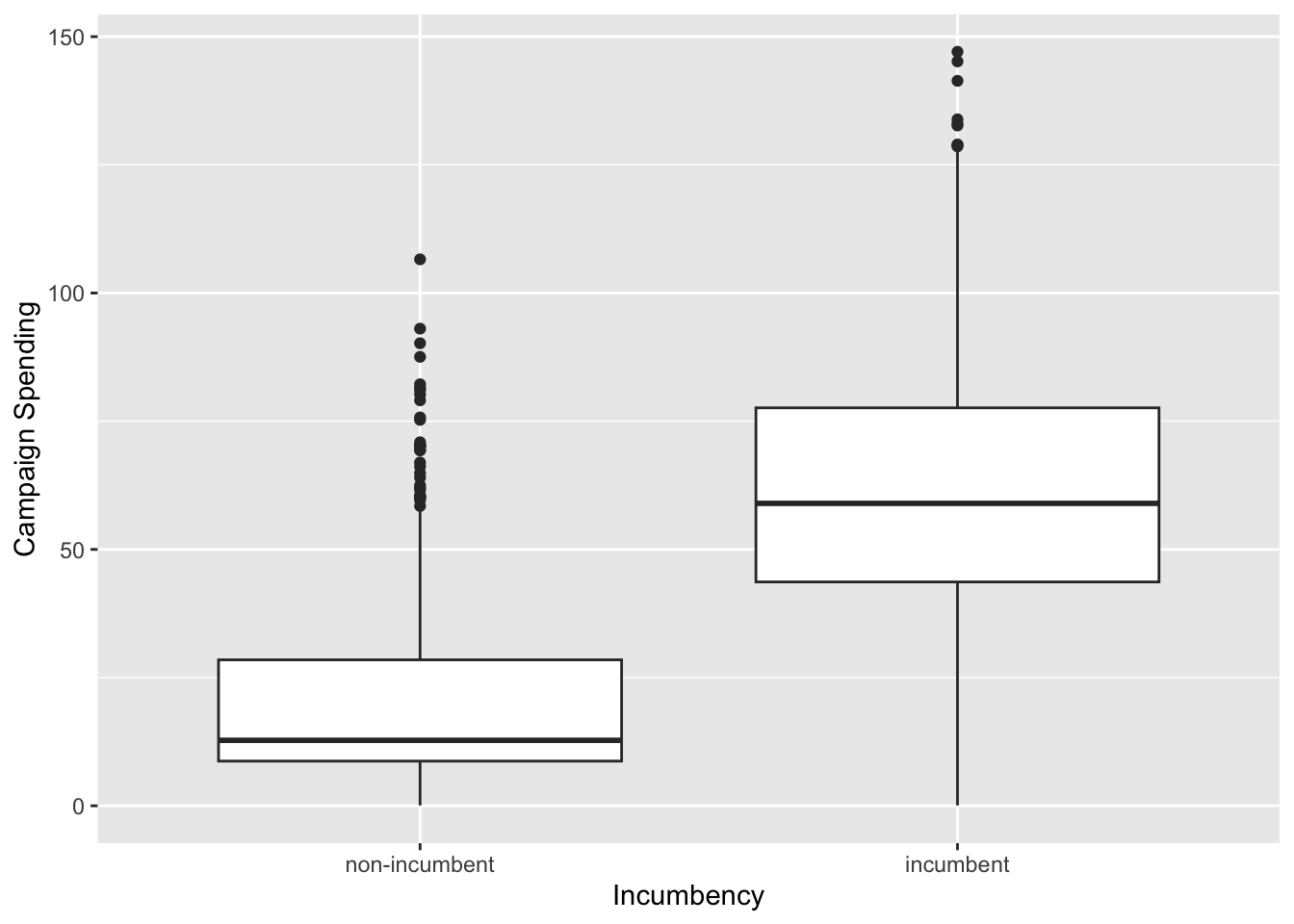
Now, let’s see if Z –> + –> Y
# numerical summary
by(je $ exp, je $ incumbent, summary)
## je$incumbent: non-incumbent
##      Min.   1st Qu.    Median      Mean   3rd Qu.      Max.
##   0.05814   8.71506  12.77014  20.89402  28.46351 106.57386
## ------------------------------------------------------------
## je$incumbent: incumbent
##      Min.   1st Qu.    Median      Mean   3rd Qu.      Max.
##   0.06008  43.65598  58.97949  62.73271  77.61213 147.05360
# graphical summary
g <- ggplot(je, aes(x = incumbent, y = exp)) + geom_boxplot()
g <- g + ylab("Campaign Spending") + xlab("Incumbency")
g
# ggsave(file="figs/csin.pdf", width=8, height=6)
We do see that Z and Y are positively related.
Now, let’s see if Z –> + –> X
# numerical summary
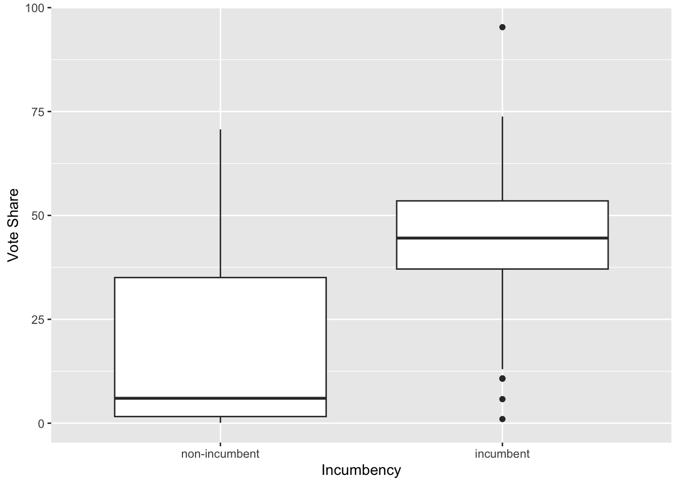
by(je $ voteshare, je $ incumbent, summary)
## je$incumbent: non-incumbent
##    Min. 1st Qu.  Median    Mean 3rd Qu.    Max.
##    0.10    1.60    6.00   16.55   35.05   70.70
## ------------------------------------------------------------
## je$incumbent: incumbent
##    Min. 1st Qu.  Median    Mean 3rd Qu.    Max.
##    1.00   37.10   44.55   45.15   53.50   95.30
# graphical summary
g <- ggplot(je, aes(x = incumbent, y = voteshare)) + geom_boxplot()
g <- g + ylab("Vote Share") + xlab("Incumbency")
g
# ggsave(file="figs/vsin.pdf", width=8, height=6)
We also see that Z and X are positively related as well. So we’d better control for this variable.
Controlling for Z using an additive model
fit.2 <- lm(voteshare ~ exp + incumbent, data = je)
stargazer(fit.1, fit.2, type = "text")
##
## =========================================================================
##                                      Dependent variable:
##                     -----------------------------------------------------
##                                           voteshare
##                                 (1)                        (2)
## -------------------------------------------------------------------------
## exp                          0.530***                   0.391***
##                               (0.017)                    (0.022)
##
## incumbentincumbent                                      12.238***
##                                                          (1.335)
##
## Constant                     7.735***                   8.384***
##                               (0.757)                    (0.734)
##
## -------------------------------------------------------------------------
## Observations                   1,124                      1,124
## R2                             0.478                      0.515
## Adjusted R2                    0.478                      0.514
## Residual Std. Error     16.042 (df = 1122)         15.480 (df = 1121)
## F Statistic         1,028.236*** (df = 1; 1122) 594.131*** (df = 2; 1121)
## =========================================================================
## Note:                                         *p<0.1; **p<0.05; ***p<0.01
We see that
(a) the second model fits the data better (look at R2 and RMSE);
(b) the slope for exp is still positive and statistically significant even after we control for incumbency status; but
(c) the slope for exp is smaller once we account for incumbency status.
This means that we indeed need to control for incumbency status. However, we suspect that this may not be enough. We thus turn to interactive models.
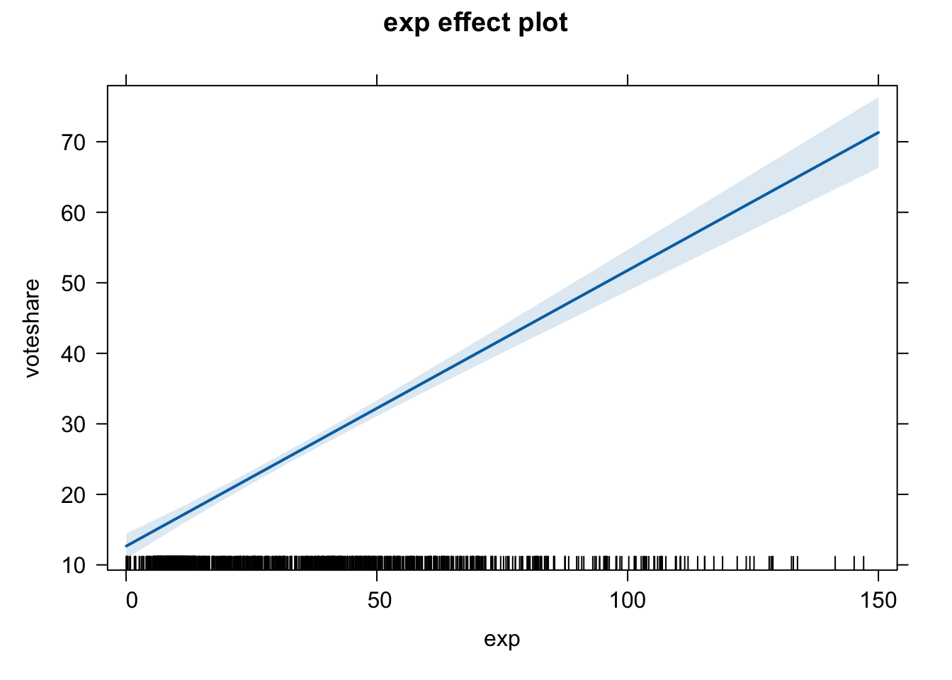
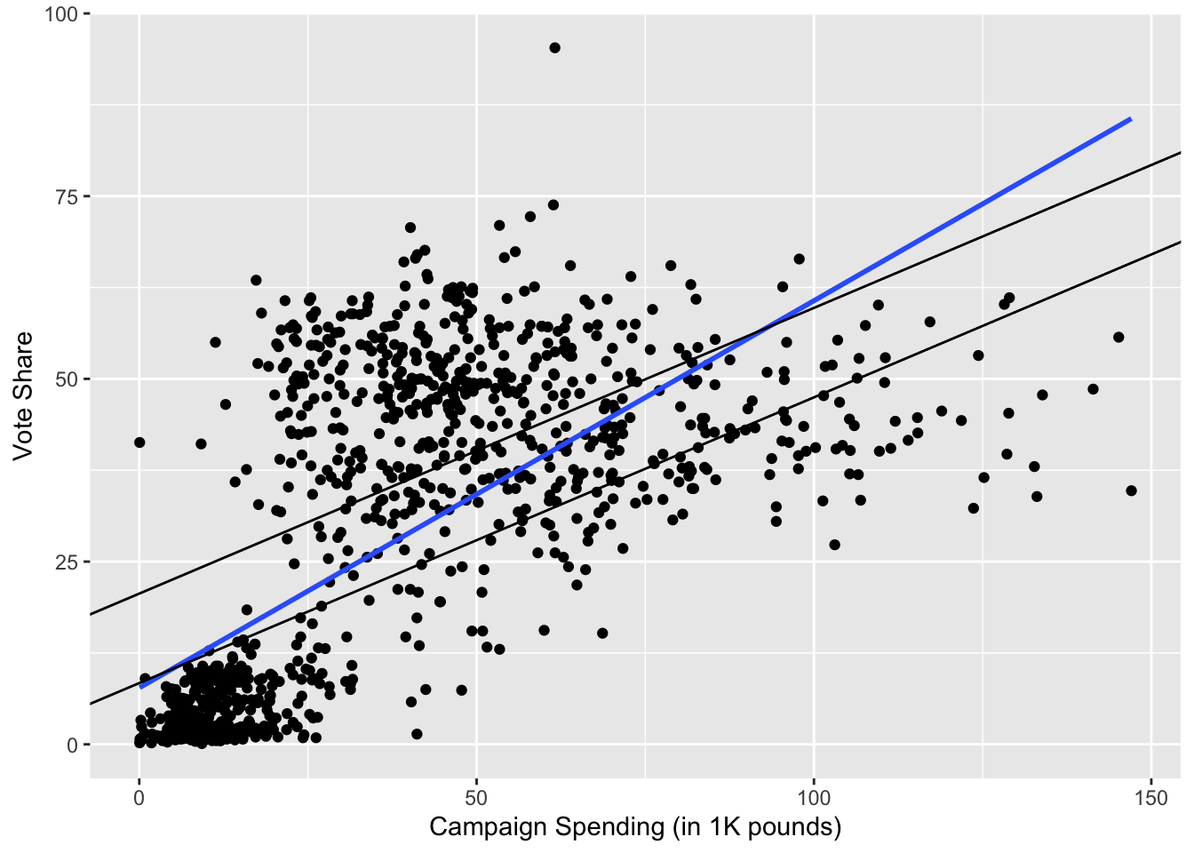
Before moving on, let’s obtain and plot the implied regression lines from the second model.
plot(effect(term = "exp", mod = fit.2))
If you want to do this with ggplot2, do the following:
g <- ggplot(je, aes(x = exp, y = voteshare)) + geom_point()
g <- g + ylab("Vote Share") + xlab("Campaign Spending (in 1K pounds)")
g <- g + geom_smooth(method = lm, alpha = 0) # implied regression line from model (1)
g <- g + geom_abline(intercept = coef(fit.2)[1], slope = coef(fit.2)[2]) # line for non-incumbent
g <- g + geom_abline(intercept = coef(fit.2)[1] + coef(fit.2)[3], slope = coef(fit.2)[2]) # line for incumbent
g
## `geom_smooth()` using formula = 'y ~ x'
# ggsave(file="figs/vsex3.pdf", width=8, height=6)
Controlling for incumbency status (interaction model)
Another way to control for Z is to estimate an interaction model, a model where not only the intercepts but also the slopes are allowed to vary depending on the values of Z.
To have an interaction term in R, we combine variables with a colon (*), as follows:
fit.3 <- lm(voteshare ~ exp + incumbent + exp*incumbent, data = je)
In the above model, the third term in the right-hand-side of the formula, exp*incumbent, is the interaction term between exp and incumbent. That is, exp:incumbent is the product of exp and incumbent.
stargazer(fit.1, fit.2, fit.3, type = "text")
##
## ======================================================================================================
##                                                      Dependent variable:
##                        -------------------------------------------------------------------------------
##                                                           voteshare
##                                    (1)                        (2)                       (3)
## ------------------------------------------------------------------------------------------------------
## exp                             0.530***                   0.391***                  0.864***
##                                  (0.017)                    (0.022)                   (0.026)
##
## incumbentincumbent                                         12.238***                 46.758***
##                                                             (1.335)                   (1.791)
##
## exp:incumbentincumbent                                                               -0.866***
##                                                                                       (0.036)
##
## Constant                        7.735***                   8.384***                  -1.502**
##                                  (0.757)                    (0.734)                   (0.721)
##
## ------------------------------------------------------------------------------------------------------
## Observations                      1,124                      1,124                     1,124
## R2                                0.478                      0.515                     0.681
## Adjusted R2                       0.478                      0.514                     0.680
## Residual Std. Error        16.042 (df = 1122)         15.480 (df = 1121)        12.548 (df = 1120)
## F Statistic            1,028.236*** (df = 1; 1122) 594.131*** (df = 2; 1121) 798.028*** (df = 3; 1120)
## ======================================================================================================
## Note:                                                                      *p<0.1; **p<0.05; ***p<0.01
Now we have results from three different models:
model (1) is the most restrictive model that relies on an assumption that exp is the only determinant of voteshare. That is, the effect of the other variables are relegated to the error term (residual). This model is justified only if there is no third variable that affects both our X and Y (which we can’t know until we actually estimate less restrictive models)
model (2) is the additive model. It seeks to control for the incumbency status by allowing incumbent and non-incumbent candidates to have different intercepts, while still assuming that the slope are the same. Note, again, that the slope for exp from model (2) does not have to be equal to the slope for exp from model (1).
model (3) is the interactive model. It allows both the intercepts and the slopes for exp to vary by the values of Z. This is the most flexible of the three models. In other words, this model relies on the least restrictive set of assumptions. It no longer assumes that the slope are the same for incumbent and non-incumbent candidates. Instead, we let the data tell us if they are the same or not.
So, what do we get?
It turns out that the third model outperforms the first two in terms of model fit, so we choose the third model.
## The regression line we estimated is:
## vs hat = -1.502 + 0.864 * exp + 46.758 * inc - 0.866 * exp * inc

## Then, the implied regression lines for non-incumbent and incumbent
## candidates are:

# non-incumbent (je $ incumbent == "non-incumbent")
# vs hat = -1.502 + 0.864 * exp + 46.758 * (0) - 0.866 * exp * (0)
#        = -1.502 + 0.864 * exp

# incumbent (je $ incumbent == "incumbent")
# vs hat = -1.502 + 0.864 * exp + 46.758 * (1) - 0.866 * exp * (1)
#        = -1.502 + 0.864 * exp + 46.758 - 0.866 * exp
#        = (-1.502 + 46.758) + (0.864 - 0.866) * exp
#        = 45.256 - 0.002 * exp
Confused much?
Whenever you run an interactive model, it would be better (and easier) to interpret the findings using graphs, as follows.
plot(effect(term = "exp:incumbent", mod = fit.3))
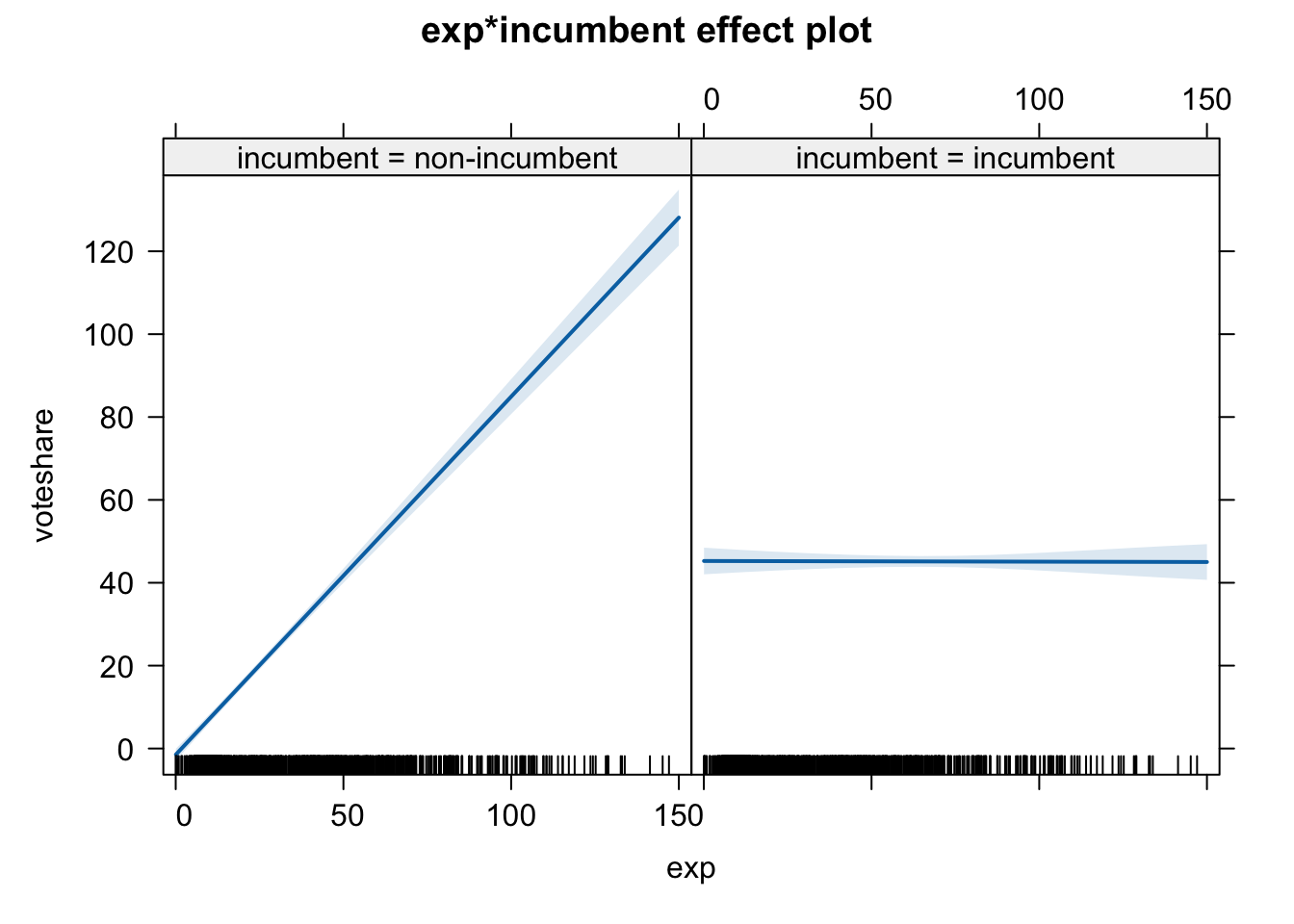
Note that we ask R to plot the effect of the interaction term exp:incumbent, then R will create two graphs that show the effect of exp on Y for different values of incumbent.
The left panel shows the relationship for non-incumbent (Y = -1.502 + 0.864 * exp), whereas the right panel shows that for incumbent (Y = 45.256 - 0.002 * exp).
We can clearly see that the effect of campaign spending is conditioned by incumbency status. The vote share of non-incumbent candidates is strongly affected by campaign spending (left panel), whereas the vote share of incumbent is hardly affected by campaign spending (right panel).
As we saw in the lecture, there is an alternative way to obtain the same implied regression lines. If we estimate the model voteshare ~ exp for the sample of incumbents and for the sample of non-incumbents separately, we would obtain the exact same results as above.
fit.4 <- lm(voteshare ~ exp, data = je[je $ incumbent == "non-incumbent",])
fit.5 <- lm(voteshare ~ exp, data = je[je $ incumbent == "incumbent",])
stargazer(fit.4, fit.5, type = "text")
##
## ==================================================================
##                                  Dependent variable:
##                     ----------------------------------------------
##                                       voteshare
##                                (1)                     (2)
## ------------------------------------------------------------------
## exp                          0.864***                -0.002
##                              (0.027)                 (0.023)
##
## Constant                     -1.502**               45.256***
##                              (0.740)                 (1.558)
##
## ------------------------------------------------------------------
## Observations                   732                     392
## R2                            0.582                  0.00001
## Adjusted R2                   0.581                  -0.003
## Residual Std. Error     12.868 (df = 730)       11.927 (df = 390)
## F Statistic         1,015.608*** (df = 1; 730) 0.005 (df = 1; 390)
## ==================================================================
## Note:                                  *p<0.1; **p<0.05; ***p<0.01
Model (1) in the table above is the results for non-incumbents. Look at the slope and the intercept. These are EXACTLY the same as the implied regression line estimates we had in line 178. Likewise, model (2) gives us the exact same results for incumbents.
So, running an interactive model where we interact ALL the independent variables with one dummy variable is mathematically equivalent to running two models for separate samples. Notice that we only have exp and incumbent as the independent variables. If we interact exp and incumbent, we can say that we interact ALL the independent variables with one dummy variable (incumbent).
Numerical x numerical interaction
As we learned in the lecture, an interaction term doesn’t have to be between a dummy and a numerical; we can interact two numerical variables.
Here, we will regress female representation (women09) on per capita GDP, ethnic fractionalization, and an interaction term between the two.
# World data
wd <- pd <- read.csv("/Users/howardliu/methodsPol/content/class/world.csv")

# 1. Additive model (for comparison)
fit.wm1 <- lm(women09 ~ frac_eth + gdp_10_thou, data = wd)

# 2. Interactive model
fit.wm2 <- lm(women09 ~ frac_eth + gdp_10_thou + frac_eth:gdp_10_thou, data = wd)

stargazer(fit.wm1, fit.wm2, type = "text")
##
## ==================================================================
##                                   Dependent variable:
##                      ---------------------------------------------
##                                         women09
##                               (1)                    (2)
## ------------------------------------------------------------------
## frac_eth                     2.406                 7.937**
##                             (3.300)                (3.697)
##
## gdp_10_thou                 3.610***               6.936***
##                             (0.880)                (1.390)
##
## frac_eth:gdp_10_thou                              -10.177***
##                                                    (3.344)
##
## Constant                   13.776***              11.275***
##                             (1.855)                (1.987)
##
## ------------------------------------------------------------------
## Observations                  166                    166
## R2                           0.095                  0.144
## Adjusted R2                  0.084                  0.128
## Residual Std. Error    10.359 (df = 163)      10.106 (df = 162)
## F Statistic          8.581*** (df = 2; 163) 9.099*** (df = 3; 162)
## ==================================================================
## Note:                                  *p<0.1; **p<0.05; ***p<0.01
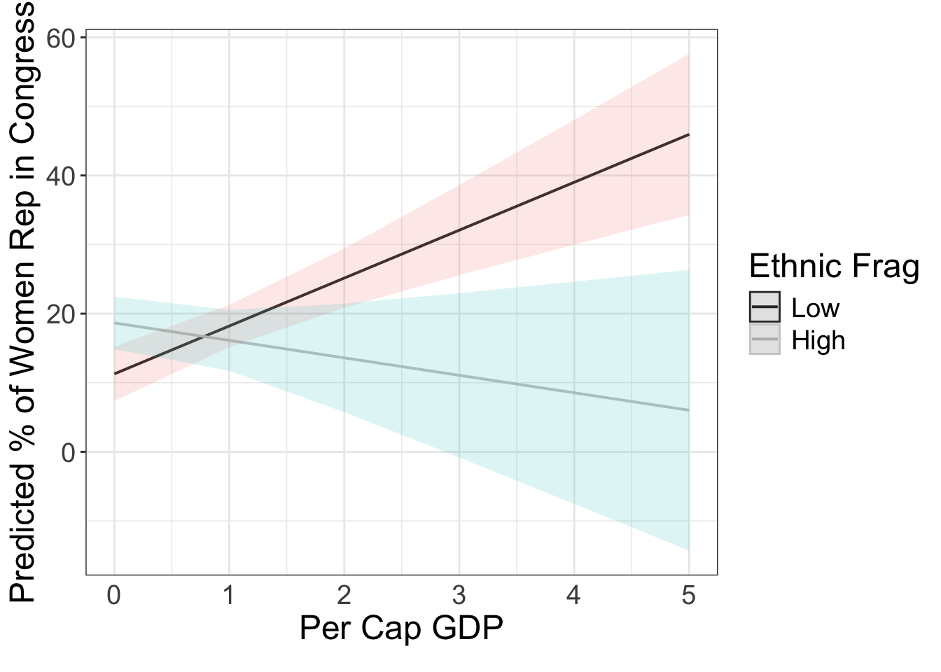
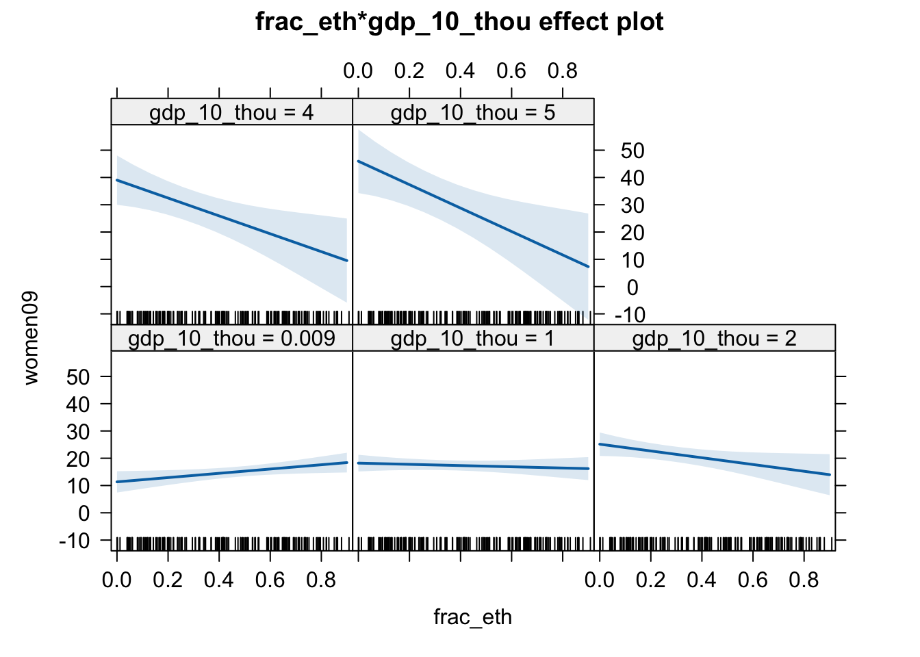
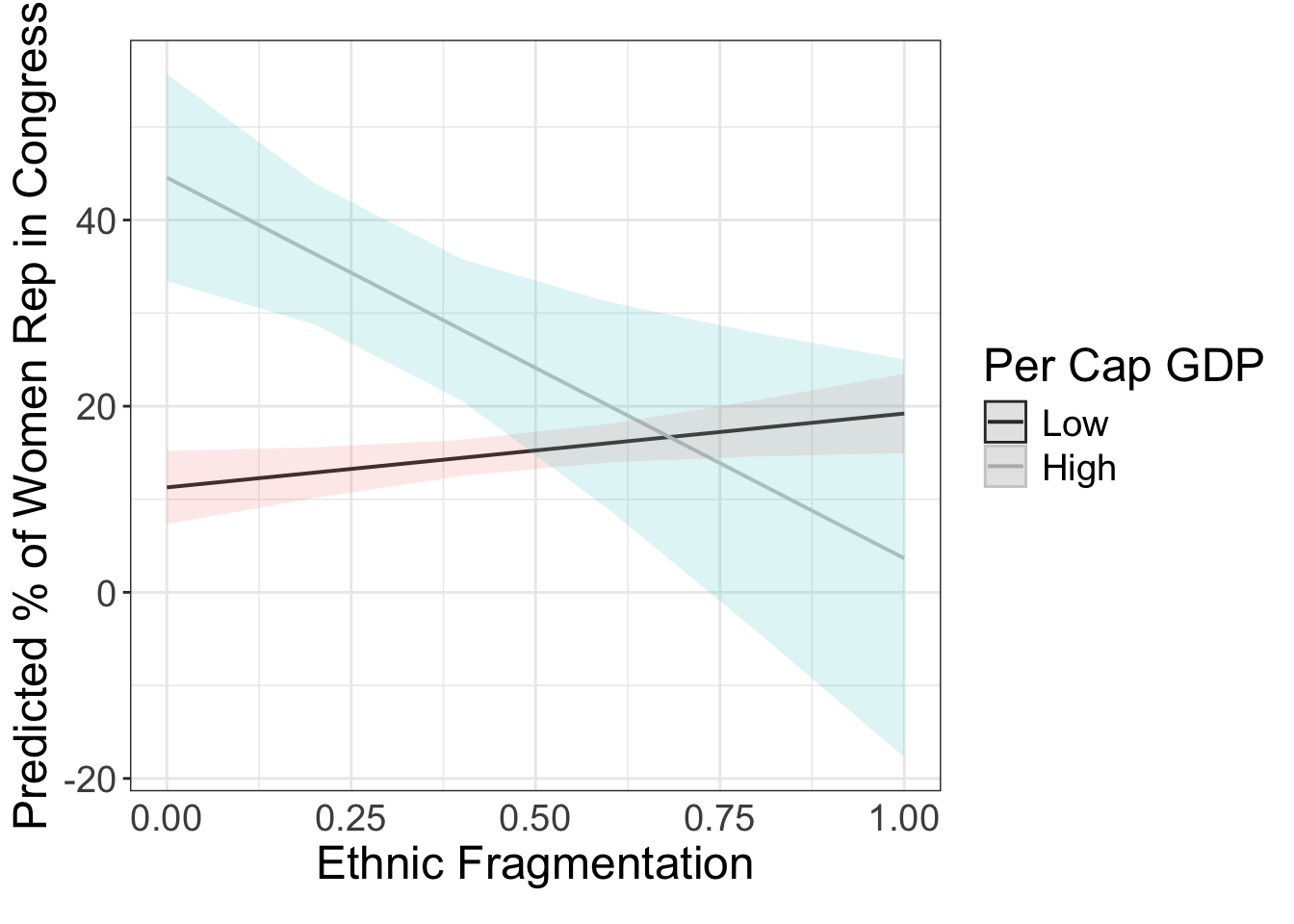
As gdp_10_thou and frac_eth are both numerical (continuous), there are infinite number of implied regression lines. So, instead of deriving them mathematically, we will turn to visual interpretation.
# pdf(file = "figs/effect_wm.pdf", width = 10, height = 5)
plot(effect(term = "frac_eth:gdp_10_thou", mod = fit.wm2))
# dev.off()
We can do a similar thing in R:
max(wd$frac_eth, na.rm =T)
## [1] 0.9302
min(wd$frac_eth, na.rm =T)
## [1] 0
max(wd$gdp_10_thou, na.rm =T)
## [1] 4.7354
min(wd$gdp_10_thou, na.rm =T)
## [1] 0.009
library(sjPlot)
##
## Attaching package: 'sjPlot'

## The following object is masked from 'package:ggplot2':
##
##     set_theme
g = plot_model( fit.wm2, type = "pred", terms = c( "frac_eth",  "gdp_10_thou[0, 4.8]"), ci.lvl = 0.95, robust = T, vcov.type = c("HC3"),bpe.style = "line" ) +
  theme_bw() +
  xlab("Ethnic Fragmentation") + ylab("Predicted % of Women Rep in Congress") +
  labs(caption = element_blank()) +
  theme( legend.justification = c(0, .5), text = element_text(size=18), axis.ticks.x=element_blank()) +
  scale_colour_grey(guide = guide_legend(title = "Per Cap GDP"), labels = c("Low", "High")) + #"Median",
  ggtitle(element_blank())
## Scale for colour is already present.
## Adding another scale for colour, which will replace the existing scale.
g
## Warning: `label` cannot be a <ggplot2::element_blank> object.
## `label` cannot be a <ggplot2::element_blank> object.
library(sjPlot)
g = plot_model( fit.wm2, type = "pred", terms = c( "gdp_10_thou", "frac_eth[0, 0.93]"), ci.lvl = 0.95, robust = T, vcov.type = c("HC3"),bpe.style = "line" ) +
  theme_bw() +
  xlab("Per Cap GDP") + ylab("Predicted % of Women Rep in Congress") +
  labs(caption = element_blank()) +
  theme( legend.justification = c(0, .5), text = element_text(size=18), axis.ticks.x=element_blank()) +
  scale_colour_grey( guide = guide_legend(title = "Ethnic Frag"), labels = c("Low", "High")) + #"Median",
  ggtitle(element_blank())
## Scale for colour is already present.
## Adding another scale for colour, which will replace the existing scale.
g
## Warning: `label` cannot be a <ggplot2::element_blank> object.
## `label` cannot be a <ggplot2::element_blank> object.
