Data Management
We learn three main things during this week’s lab session:
- Loading packages
- Importing data sets from a file
- Summarizing categorical and numerical data
0. Preparation (Creating an R project)
Before we begin, do the following:
-
If you haven’t done so already, create a folder named “POLI502” somewhere on your computer (could be on your desktop, documents folder, etc.)
-
Download all the files for today from Blackboard, including POLI502-week5-JointExercise.R, POLI502-week5-IndividualExercise.R, world.csv, world codebook.pdf
-
Move all the four files you downloaded to your own POLI502 folder.
-
Create a R project in the POLI502 folder if you haven’t done so already
1. Loading R packages
We have been using some R functions such as summary(), data.frame(), sqrt(), etc. These simple functions come with the base R installation and so we can use them without doing any additional installation.
One of the great advantages of R is the availability of “packages” – a collection of additional functions. To use a package, we need to do two things:
- Install it
- Load it
Installation must be done just once per computer. For example, once you install a package called ggplot2 to your computer, you won’t need to install it ever again. However, you still need to load the package each time you start a new R session.
(1) Installing a package
To install an R package, we use the install.packages function.
# install.packages("ggplot2", dependencies = TRUE)
ggplot2 is the name of the package we install. We put the dependencies = TRUE option here because we want to install all the additional packages that ggplot2 depends on.
Some packages depend on other packages. For example, the ggplot2 package depends on eight other packages (plyr, digest, grid, gtable, reshape2, scales, proto, and MASS), each of which might also depend on yet other packages. Loading the ggplot2 package requires that we also load all the packages that it depends on, which means that we need to install all these packages. The dependencies = TRUE option does exactly that.
Installation might take a while, but the good news is that you don’t need to do this again for ggplot2 (Of course, you may have to install some other packages in the future).
Once the installation is done, you can now load the ggplot2 package.
library(ggplot2)
If you don’t get any error message, it means you have successfully loaded this package.
Remember that loading must be done every time we start R (R studio).
(2) Loading a package
To load a package, we use the library function. Let’s load a package called ggplot2, which contains a lot of graphic functions.
library(ggplot2)
What happened on your computer?
If you are using your own computer, you probably got an error message saying Error in library(ggplot2) : there is no package called ‘ggplot2’.
This happened because we haven’t done (1).
If, on the other hand, you are using a lab computer, you probably didn’t get any error message. This is because someone has already installed this package to the computer you are using. Remember we need to install a package once per computer.
2. Importing data sets from a file
We have learned how to work with data.frame objects last week. We even created a mini data set using the data.frame function. In practice, we work with data sets that are much larger than the mini data set we created. Moreover, we usually import such data sets from a file, not by typing in information on our own. To read in (=import) a data set from a file, we use read.XXX functions, such as
read.csv: Comma-separated text fileread.table: Tab-separated text fileread.dta: Stata fileread.spss: SPSS fileread.xlsx: Excel file
We will use the read.csv function today. We will learn others in the future.
Let’s use the read.csv function and import the “World” data set we discussed in the lecture.
# path = "/Users/howardliu/Library/CloudStorage/Dropbox/myjobs/UofSC_South-carolina/SC_teaching/POLI502/502_week5_measurement/lab-week5-describe-data/"
# world.data <- read.csv(paste0(path, "world.csv"))
world.data <- read.csv("world.csv")
What happened on your computer?
If you don’t get any error message, that’s perfect. You have successfully imported a data set from the world.csv file.
If, on other other hand, you get an error message that starts with Error in file(file, "rt") : cannot open the connection, that could be because of one or more of the following reasons:
- You haven’t downloaded the world.csv file from Blackboard or from the course website;
- You haven’t moved the world.csv file to the POLI502 folder;
- You have done both (1) and (2), but R doesn’t know where POLI502 is.
Let’s first do (1) and (2) if you haven’t done so. Now we will see how to resolve (3).
Setting the path
When you do some file operations in R (such as loading a data set from a file, or saving data, graphs, or outputs into a file), we need to tell R the exact location (address) of the file.
Locations on a computer are called “path”. A path is like an address. It identifies the location of files and folders on a computer.
When using functions such as read.csv, R looks for files contained in one folder and one folder only. The folder that R thinks R is located currently is called “current directory” or “working directory”.
“Directory” is just another name for “folder”. So, the working directory refers to the folder that R searches when trying to open a file.
When you open R Studio by double-clicking on a script file (such as the present file POLI502-week5-JointExercise.R), the working directory is automatically set to the folder that contains the script file.
Therefore, if you have opened this 502-week5-JointExercise.R file saved today, then the working directory has been correctly set to POLI502.
If not, we need to change it.
To find out what folder R is currently residing, we use the getwd function, short for “get W(orking) D(irectory)”
getwd() this is the magic working in a R project; you don’t need to setwd each time and it saves time for your collaborator
If you are on a lab computer, R will tell you something like: m:/pc/desktop/POLI502
If you are on a Mac computer, R will tell you something like: Users/howardliu/Desktop/POLI502 or Users/howardliu/Documents/POLI502
To change the working directory, we use the setwd function, short for “set W(orking) D(irectory)”
If you are on a lab computer, execute the following. Do not execute it if you are on your own computer.
# setwd("m:/pc/desktop/POLI502")
If you are using your own Mac computer, execute the following: You need to replace “daina” with your own username.You may also need to replace “Desktop” with “Documents” or something, depending on where you created the POLI502 folder.
# setwd("/Users/howardliu/Dropbox/POLI502")
If you are using your own Windows computer, the exact path would depend on how your computer is configured, so you probably want to ask for your TA’s help.
One option is to close R Studio once, and re-open it by double-clicking on the POLI502-week5-JointExercise.R file.
Now, let’s see if the path is set correctly.
getwd()
## [1] "/Users/howardliu/methodsPol/content/class"
If it shows the location of the POLI502 folder that contains the world.csv file, we should be able to execute the following again.
# View(world.data)
Look what we are doing above. We are creating a new object named world.data and its contents is the result of applying the read.csv function.
Note: If you load data in a quarto doc (.qmd), quarto uses a relative directory, meaning it doesn’t allow you to set a different working dir for your data file. Currently, you would need to save the data file in the same folder as your quarto file so the data can be loaded.
Understanding pipe operator %>% in R
Nice reference on pipes here
The pipe operator makes it possible to easily chain a sequence of calculations.
first, install it from this package
library(magrittr)

x <- -300

round((sqrt(abs(x))))
## [1] 17
x <- c(0.109, 0.359, 0.63, 0.996, 0.515, 0.142, 0.017, 0.829, 0.907)
Compute the logarithm of x, return suitably lagged and iterated differences, compute the exponential function and round the result
round(exp(diff(log(x))), 1)
## [1] 3.3 1.8 1.6 0.5 0.3 0.1 48.8 1.1
round(exp(diff(log(x))), 1)
## [1] 3.3 1.8 1.6 0.5 0.3 0.1 48.8 1.1
x %>% log %>% diff %>% exp %>% round(., 1)
## [1] 3.3 1.8 1.6 0.5 0.3 0.1 48.8 1.1
The hotkey for %>% is Command + shift + m
In the following, I’ll show you situations where using pipes makes your life easier
Difference between base R |> (native pipes) and magrittr %>% (pipes)
While |> and %>% behave identically for simple cases, there are a few crucial differences. These are most likely to affect you if you’re a long-term user of %>% who has taken advantage of some of the more advanced features. But they’re still good to know about even if you’ve never used %>% because you’re likely to encounter some of them when reading wild-caught code
%>%allows you to drop the parentheses when calling a function with no other arguments;|>always requires the parentheses.
# library(magrittr)
library(tidyverse)
## ── Attaching core tidyverse packages ──────────────────────── tidyverse 2.0.0 ──
## ✔ dplyr     1.1.4     ✔ readr     2.1.5
## ✔ forcats   1.0.0     ✔ stringr   1.5.1
## ✔ lubridate 1.9.3     ✔ tibble    3.2.1
## ✔ purrr     1.0.2     ✔ tidyr     1.3.1
## ── Conflicts ────────────────────────────────────────── tidyverse_conflicts() ──
## ✖ tidyr::extract()   masks magrittr::extract()
## ✖ dplyr::filter()    masks stats::filter()
## ✖ dplyr::lag()       masks stats::lag()
## ✖ purrr::set_names() masks magrittr::set_names()
## ℹ Use the conflicted package (<http://conflicted.r-lib.org/>) to force all conflicts to become errors
world.data %>%
  filter(!is.na(democ_regime)) %>%
   .$country %>%
  head()
## [1] "Afghanistan"       "Albania"           "Algeria"
## [4] "Andorra"           "Angola"            "Antigua & Barbuda"
world.data |>
  filter(!is.na(democ_regime)) |>
  head()
##             country       colony confidence decentralization dem_other
## 1       Afghanistan           UK         NA               NA      10.5
## 2           Albania Soviet Union   49.33593             0.74      63.0
## 3           Algeria       France   52.05573               NA      40.8
## 4           Andorra        Spain         NA               NA     100.0
## 5            Angola     Portugal         NA               NA      40.8
## 6 Antigua & Barbuda           UK         NA               NA      87.5
##   dem_other5 democ_regime    district_size3 durable effectiveness      enpp_3
## 1        10%           No     single member       4      13.71158
## 2 Approx 60%          Yes                         3      35.46099 1-3 parties
## 3 Approx 40%           No 6 or more members       5      32.62411
## 4       100%          Yes                        NA      78.72340
## 5 Approx 40%           No                         3      19.14894
## 6 Approx 90%          Yes     single member      NA      59.81088 1-3 parties
##           eu fhrate04_rev fhrate08_rev frac_eth frac_eth3 free_business
## 1 Not member          2.5            3   0.7693      High            NA
## 2 Not member            5            8   0.2204       Low          68.0
## 3 Not member          2.5            3   0.3394    Medium          71.2
## 4 Not member    Most free           12   0.7139      High            NA
## 5 Not member          2.5            3   0.7867      High          43.4
## 6 Not member            6           10   0.1643       Low            NA
##   free_corrupt free_finance free_fiscal free_govspend free_invest free_labor
## 1           NA           NA          NA            NA          NA         NA
## 2           34           70        92.6          74.2          70       52.1
## 3           32           30        83.5          73.4          45       56.4
## 4           NA           NA          NA            NA          NA         NA
## 5           19           40        85.1          62.8          35       45.2
## 6           NA           NA          NA            NA          NA         NA
##   free_monetary free_overall free_property free_trade gdp08 gdp_10_thou
## 1            NA           NA            NA         NA  30.6          NA
## 2          78.7         66.0            35       85.8  24.3      0.1535
## 3          77.2         56.9            30       70.7 276.0      0.1785
## 4            NA           NA            NA         NA    NA          NA
## 5          62.6         48.4            20       70.4 106.3      0.0857
## 6            NA           NA            NA         NA    NA      1.0449
##   gdp_cap2 gdp_cap3 gdppcap08 gender_equal3 gini04 gini08   hi_gdp indy
## 1                          NA                   NA     NA          1919
## 2      Low   Middle      7715                 28.2   31.1  Low GDP 1991
## 3      Low   Middle      8033                 35.3   35.3  Low GDP 1962
## 4                          NA                   NA     NA          1278
## 5      Low   Middle      5899                   NA     NA  Low GDP 1975
## 6     High     High        NA                   NA     NA High GDP 1981
##         oecd  old2006  old2003     pmat12_3    pop03 pop08    pop08_3
## 1 Not member       NA       NA                    NA  27.4 >=16.8 mil
## 2 Not member 8.479821 7.278363 Low post-mat  3169064   3.1  <=4.3 mil
## 3 Not member 4.578136 4.045199              31832610  34.4 >=16.8 mil
## 4 Not member       NA       NA                 66000    NA
## 5 Not member 2.450295 2.930542              13522110  18.0 >=16.8 mil
## 6 Not member       NA 8.186610                 78580    NA
##            popcat3 pr_sys protact3        regime_type3      region sources
## 1 Moderate (1-29m)     No                 Dictatorship Middle East      NA
## 2 Moderate (1-29m)     No Moderate Parliamentary democ  C&E Europe      NA
## 3 Moderate (1-29m)    Yes                 Dictatorship      Africa      NA
## 4 Small (under 1m)     No          Parliamentary democ   W. Europe      NA
## 5 Moderate (1-29m)    Yes                 Dictatorship      Africa      NA
## 6 Small (under 1m)     No          Parliamentary democ  S. America      NA
##          typerel unions urban03 urban06 vi_rel3 votevap00s women05 women09
## 1         Muslim     NA      NA   23.28                 NA      NA    27.7
## 2         Muslim     NA 44.2390   46.14  20-50%      59.56     6.4    16.4
## 3         Muslim     NA 58.8302   63.94    >50%         NA      NA     7.7
## 4 Roman Catholic     NA 91.7404   90.28              20.95    14.3    35.7
## 5 Roman Catholic     NA 36.1806   53.96                 NA      NA    37.3
## 6     Protestant     NA 37.7566   39.60              76.34    10.5    10.5
##   womyear       womyear2  yng2003  young06
## 1      NA                      NA       NA
## 2    1920 1944 or before 27.34834 26.35428
## 3    1962     After 1944 33.91887 28.94154
## 4    1973     After 1944       NA       NA
## 5    1975     After 1944 47.62524 46.32196
## 6    1951     After 1944 20.66509       NA
# .$country
%>%allows you to start a pipe with.to create a function rather than immediately executing the pipe; this is not supported by the base pipe.
Exploring a data set
Whenever you read in a data set from a file, it’s always a good idea to take a look at it first to have an idea about what it looks like. There are a few functions that will let us take a look at the data set. The dim function tells us the dimension (the number of rows and the number of columns)
dim(world.data)
## [1] 191 62
So this contains 191 rows (observations) and 62 columns (variables)
The head and tail functions let us see the first or last 5 rows of the data set.
# world.data
# head(world.data,10)

# tail(world.data,8)
Or we can do this using the square brackets
world.data[1:10, 1:5]
##              country       colony confidence decentralization dem_other
## 1        Afghanistan           UK         NA               NA      10.5
## 2            Albania Soviet Union  49.335926             0.74      63.0
## 3            Algeria       France  52.055735               NA      40.8
## 4            Andorra        Spain         NA               NA     100.0
## 5             Angola     Portugal         NA               NA      40.8
## 6  Antigua & Barbuda           UK         NA               NA      87.5
## 7          Argentina        Spain   7.299325             2.40      87.5
## 8            Armenia Soviet Union  27.132735               NA      63.0
## 9          Australia           UK  46.838886             1.74      58.3
## 10           Austria        Other  49.680190             1.81     100.0
This tells R to show the first 10 rows and first 5 columns. We can easily see that country is the unit of observation. We can also see that there are variables such as colony, confidence, decentralization, and dem_other.
When working with a large data set like this one, you may want to use the spreadsheet view (just like Excel). To do so, we use the View function, which opens a spreadsheet tab in the script pane.
# View(world.data)
3. Summarizing data
Now we will use numerical and graphical methods to summarize data. As we learned in the lecture, we will need different methods for different types of data (categorical or numerical).
Categorical variables
As we saw in the lecture, there is a variable called “colony” in the data set that records the former colonial master country for each observation. Let’s see how to summarize the information contained in this variable.
To access a variable included in a data frame object, we use the $ symbol.
# world.data $ colony
Now R shows the values of this variable for all the 191 observations. We can see that this variable takes values such as UK, Soviet Union, France, etc. To see what value each country (each row) takes, we may want to see the “country” variable and the “colony” variables at the same time. Since the “country” variable is stored in the first column and the “colony” variable in the second column, we can do the following:
# world.data[, 1:2]
This shows the first and second columns for all rows. Alternatively, we can do the following to get the same output.
world.data[ c("country", "colony") ]
##                      country       colony
## 1                Afghanistan           UK
## 2                    Albania Soviet Union
## 3                    Algeria       France
## 4                    Andorra        Spain
## 5                     Angola     Portugal
## 6          Antigua & Barbuda           UK
## 7                  Argentina        Spain
## 8                    Armenia Soviet Union
## 9                  Australia           UK
## 10                   Austria        Other
## 11                Azerbaijan Soviet Union
## 12                   Bahamas           UK
## 13                   Bahrain           UK
## 14                Bangladesh        Other
## 15                  Barbados           UK
## 16                   Belarus Soviet Union
## 17                   Belgium  Netherlands
## 18                    Belize           UK
## 19                     Benin       France
## 20                    Bhutan        Other
## 21                   Bolivia        Spain
## 22                    Bosnia Soviet Union
## 23                  Botswana           UK
## 24                    Brazil     Portugal
## 25         Brunei Darussalam           UK
## 26                  Bulgaria Soviet Union
## 27              Burkina Faso       France
## 28                   Burundi      Belgium
## 29                  Cambodia       France
## 30                  Cameroon       France
## 31                    Canada           UK
## 32                Cape Verde     Portugal
## 33  Central African Republic       France
## 34                      Chad       France
## 35                     Chile        Spain
## 36                     China         none
## 37                  Colombia       France
## 38                   Comoros       France
## 39         Congo Brazzaville       France
## 40            Congo Kinshasa      Belgium
## 41                Costa Rica        Spain
## 42             Cote d'Ivoire       France
## 43                   Croatia Soviet Union
## 44                      Cuba        Spain
## 45                    Cyprus           UK
## 46            Czech Republic Soviet Union
## 47                   Denmark         none
## 48                  Djibouti       France
## 49                  Dominica           UK
## 50             Dominican Rep        Other
## 51                   Ecuador        Spain
## 52                     Egypt           UK
## 53               El Salvador        Spain
## 54         Equatorial Guinea        Spain
## 55                   Eritrea        Other
## 56                   Estonia Soviet Union
## 57                  Ethiopia         none
## 58                      Fiji           UK
## 59                   Finland         none
## 60                    France       France
## 61                     Gabon       France
## 62                    Gambia           UK
## 63                   Georgia Soviet Union
## 64                   Germany         none
## 65                     Ghana           UK
## 66                    Greece      Ottoman
## 67                   Grenada           UK
## 68                 Guatemala        Spain
## 69             Guinea-Bissau        Spain
## 70                    Guinea     Portugal
## 71                    Guyana           UK
## 72                     Haiti       France
## 73                  Honduras        Spain
## 74                   Hungary Soviet Union
## 75                   Iceland         none
## 76                     India           UK
## 77                 Indonesia  Netherlands
## 78                      Iran         none
## 79                      Iraq           UK
## 80                   Ireland           UK
## 81                    Israel           UK
## 82                     Italy         none
## 83                   Jamaica           UK
## 84                     Japan         none
## 85                    Jordan           UK
## 86                Kazakhstan Soviet Union
## 87                     Kenya           UK
## 88                  Kiribati           UK
## 89               Korea North        Other
## 90               Korea South        Other
## 91                    Kuwait           UK
## 92                Kyrgyzstan Soviet Union
## 93                      Laos       France
## 94                    Latvia Soviet Union
## 95                   Lebanon       France
## 96                   Lesotho           UK
## 97                   Liberia           UK
## 98                     Libya        Other
## 99             Liechtenstein         none
## 100                Lithuania Soviet Union
## 101               Luxembourg  Netherlands
## 102                Macedonia Soviet Union
## 103               Madagascar       France
## 104                   Malawi           UK
## 105                 Malaysia           UK
## 106                 Maldives           UK
## 107                     Mali       France
## 108                    Malta           UK
## 109         Marshall Islands         none
## 110               Mauritania       France
## 111                Mauritius           UK
## 112                   Mexico        Spain
## 113     Micronesia, Fed Stat         none
## 114                  Moldova Soviet Union
## 115                   Monaco         none
## 116                 Mongolia        Other
## 117                  Morocco       France
## 118               Mozambique     Portugal
## 119          Myanmar (Burma)           UK
## 120                  Namibia        Other
## 121                    Nauru           UK
## 122                    Nepal         none
## 123              Netherlands        Spain
## 124              New Zealand           UK
## 125                Nicaragua        Spain
## 126                    Niger       France
## 127                  Nigeria           UK
## 128                   Norway         none
## 129                     Oman     Portugal
## 130                 Pakistan           UK
## 131                    Palau         none
## 132                   Panama        Spain
## 133         Papua New Guinea        Other
## 134                 Paraguay        Spain
## 135                     Peru        Spain
## 136              Philippines        Spain
## 137                   Poland Soviet Union
## 138                 Portugal     Portugal
## 139                    Qatar           UK
## 140                  Romania Soviet Union
## 141                   Russia Soviet Union
## 142                   Rwanda      Belgium
## 143               San Marino         none
## 144                 Sao Tome     Portugal
## 145             Saudi Arabia           UK
## 146                  Senegal       France
## 147               Seychelles           UK
## 148             Sierra Leone           UK
## 149                Singapore        Other
## 150                 Slovakia Soviet Union
## 151                 Slovenia Soviet Union
## 152          Solomon Islands           UK
## 153                  Somalia           UK
## 154             South Africa           UK
## 155                    Spain        Spain
## 156                Sri Lanka           UK
## 157        St. Kitts & Nevis           UK
## 158                St. Lucia           UK
## 159  St. Vincent & Grenadine           UK
## 160                    Sudan           UK
## 161                 Suriname  Netherlands
## 162                Swaziland           UK
## 163                   Sweden         none
## 164              Switzerland         none
## 165                    Syria       France
## 166                   Taiwan        Other
## 167               Tajikistan Soviet Union
## 168                 Tanzania           UK
## 169                 Thailand         none
## 170                     Togo       France
## 171                    Tonga           UK
## 172                 Trinidad           UK
## 173                  Tunisia       France
## 174                   Turkey      Ottoman
## 175             Turkmenistan Soviet Union
## 176                   Tuvalu           UK
## 177                      UAE           UK
## 178                   Uganda           UK
## 179                  Ukraine Soviet Union
## 180           United Kingdom           UK
## 181            United States           UK
## 182                  Uruguay        Other
## 183               Uzbekistan Soviet Union
## 184                  Vanuatu       France
## 185                Venezuela        Spain
## 186                  Vietnam       France
## 187            Western Samoa        Other
## 188                    Yemen           UK
## 189      Serbia & Montenegro Soviet Union
## 190                   Zambia           UK
## 191                 Zimbabwe           UK
You can see which country was formerly colonized by which country.
Now, going back to summarizing the colony variable, we will create what’s called a frequency table to summarize a nominal-level variable like this.
This will summarize this variable in a more concise way so we can easily see things like what are the “typical” values, how frequent these typical values appear, etc.
One way to create a frequency table is to use the table function, as follows
table(world.data $ colony)
##
##      Belgium       France  Netherlands         none        Other      Ottoman
##            3           28            4           20           15            2
##     Portugal Soviet Union        Spain           UK
##            8           27           21           63
Alternatively, we can also use the summary function as well:
summary(world.data $ colony)
##    Length     Class      Mode
##       191 character character
The output above nicely summarizes the information contained in the colony variable. We can see the (raw) frequencies with which each value is observed in the data set. For example, there are 3 observations (countries) that are former colonies of Belgium, 28 former colonies of France, 4 former colonies of the Netherlands, etc.
To make it more like the frequency table you saw in the lecture slide, we can make it vertical using the data.frame function
data.frame( table(world.data $ colony) )
##            Var1 Freq
## 1       Belgium    3
## 2        France   28
## 3   Netherlands    4
## 4          none   20
## 5         Other   15
## 6       Ottoman    2
## 7      Portugal    8
## 8  Soviet Union   27
## 9         Spain   21
## 10           UK   63
tb <- world.data $ colony %>% table %>% data.frame()
Another way to summarize the information contained in a nominal-level variable is to create a bar chart, which is a graphical representation of a frequency table.
ggplot(world.data, aes(x = colony)) + geom_bar()
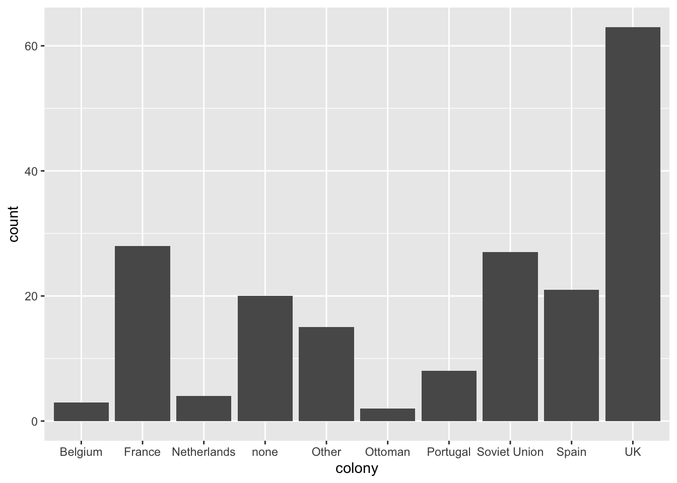
The first part tells R that world.data is the name of the data frame object that contains a variable(s) we want to plot.
The second part, the aes option (short for aesthetic) tells R which variable(s) we want to plot. We don’t need to enclose variable names with ““.
Finally, the last part, + geom_bar(), tells R that we want a bar chart. We will use geom_histogram() to create a histogram, geom_boxplot to create a box plot, geom_points() to create a scatterplot, etc. (More on this next week).
Numerical variables
This data set also contains a number of numerical variables. One of them is called “women09”, which we saw in the lecture.
world.data $ women09 %>% class
## [1] "numeric"
This variable records the percentage of women in the lower house of parliament for each country, measured in the year 2009.
To see what value each country has, we can do
# world.data[ c("country", "women09") ]
Let’s now summarize this variable. To summarize the information contained in a numeric (interval-level) variable like this one, we identify the central tendency (mean & median) and dispersion (range, inter-quartile range, standard deviation, variance), as we learned in the lecture.
The summary function gives us summary values including the five number summary mean, and the number of observations with missing values.
summary(world.data $ women09)
##    Min. 1st Qu.  Median    Mean 3rd Qu.    Max.    NA's
##    0.00    9.70   15.55   17.18   22.95   56.30      11
# Min.    = Q0 = minimum      = 0th percentile
# 1st Qu. = Q1 = 1st quartile = 25th percentile = median of the lower half of the data
# Median  = Q2 = median       = 50th percentile
# Mean         = mean (average)
# 3rd Qu. = Q3 = 3rd quartile = 75th percentile = median of the upper half of the data
# Max.    = Q4 = 4th quartile = 100th percentile = maximum value
If we just want mean or median, we can use the mean and median functions. However, it won’t work if the variable contains some missing values
mean(world.data $ women09)
## [1] NA
median(world.data $ women09)
## [1] NA
What is a missing value? Look at the data on women09 again.
world.data[ c("country", "women09") ]
##                      country women09
## 1                Afghanistan    27.7
## 2                    Albania    16.4
## 3                    Algeria     7.7
## 4                    Andorra    35.7
## 5                     Angola    37.3
## 6          Antigua & Barbuda    10.5
## 7                  Argentina    41.6
## 8                    Armenia     8.4
## 9                  Australia    26.7
## 10                   Austria    27.9
## 11                Azerbaijan    11.4
## 12                   Bahamas    12.2
## 13                   Bahrain     2.5
## 14                Bangladesh    18.6
## 15                  Barbados    10.0
## 16                   Belarus    31.8
## 17                   Belgium    35.3
## 18                    Belize     0.0
## 19                     Benin    10.8
## 20                    Bhutan     8.5
## 21                   Bolivia    16.9
## 22                    Bosnia    11.9
## 23                  Botswana    11.1
## 24                    Brazil     9.0
## 25         Brunei Darussalam      NA
## 26                  Bulgaria    20.8
## 27              Burkina Faso    15.3
## 28                   Burundi    30.5
## 29                  Cambodia    16.3
## 30                  Cameroon    13.9
## 31                    Canada    22.1
## 32                Cape Verde    18.1
## 33  Central African Republic    10.5
## 34                      Chad     5.2
## 35                     Chile    15.0
## 36                     China    21.3
## 37                  Colombia     8.4
## 38                   Comoros     3.0
## 39         Congo Brazzaville      NA
## 40            Congo Kinshasa      NA
## 41                Costa Rica    36.8
## 42             Cote d'Ivoire     8.9
## 43                   Croatia    20.9
## 44                      Cuba    43.2
## 45                    Cyprus    14.3
## 46            Czech Republic    15.5
## 47                   Denmark    38.0
## 48                  Djibouti    13.8
## 49                  Dominica    18.8
## 50             Dominican Rep    19.7
## 51                   Ecuador    32.3
## 52                     Egypt     1.8
## 53               El Salvador    19.0
## 54         Equatorial Guinea    10.0
## 55                   Eritrea    22.0
## 56                   Estonia    20.8
## 57                  Ethiopia    21.9
## 58                      Fiji      NA
## 59                   Finland    41.5
## 60                    France    18.2
## 61                     Gabon    16.7
## 62                    Gambia     9.4
## 63                   Georgia     5.1
## 64                   Germany    32.8
## 65                     Ghana     8.3
## 66                    Greece    14.7
## 67                   Grenada    13.3
## 68                 Guatemala    12.0
## 69             Guinea-Bissau    10.0
## 70                    Guinea      NA
## 71                    Guyana    30.0
## 72                     Haiti     4.1
## 73                  Honduras    23.4
## 74                   Hungary    11.1
## 75                   Iceland    42.9
## 76                     India    10.7
## 77                 Indonesia    18.2
## 78                      Iran     2.8
## 79                      Iraq    25.5
## 80                   Ireland    13.3
## 81                    Israel    17.5
## 82                     Italy    21.3
## 83                   Jamaica    13.3
## 84                     Japan    11.3
## 85                    Jordan     6.4
## 86                Kazakhstan    15.9
## 87                     Kenya     9.8
## 88                  Kiribati     4.3
## 89               Korea North    15.6
## 90               Korea South    13.7
## 91                    Kuwait     7.7
## 92                Kyrgyzstan    25.6
## 93                      Laos    25.2
## 94                    Latvia    20.0
## 95                   Lebanon     3.1
## 96                   Lesotho    25.0
## 97                   Liberia    12.5
## 98                     Libya     7.7
## 99             Liechtenstein    24.0
## 100                Lithuania    17.7
## 101               Luxembourg    20.0
## 102                Macedonia    28.3
## 103               Madagascar      NA
## 104                   Malawi    20.8
## 105                 Malaysia    10.8
## 106                 Maldives     6.5
## 107                     Mali    10.2
## 108                    Malta     8.7
## 109         Marshall Islands     3.0
## 110               Mauritania    22.1
## 111                Mauritius    17.1
## 112                   Mexico    28.2
## 113     Micronesia, Fed Stat     0.0
## 114                  Moldova      NA
## 115                   Monaco    25.0
## 116                 Mongolia     4.0
## 117                  Morocco    10.5
## 118               Mozambique    34.8
## 119          Myanmar (Burma)      NA
## 120                  Namibia    26.9
## 121                    Nauru     0.0
## 122                    Nepal    33.2
## 123              Netherlands    41.3
## 124              New Zealand    33.6
## 125                Nicaragua    18.5
## 126                    Niger    12.4
## 127                  Nigeria     7.0
## 128                   Norway    38.2
## 129                     Oman     0.0
## 130                 Pakistan    22.5
## 131                    Palau     0.0
## 132                   Panama     8.5
## 133         Papua New Guinea     0.9
## 134                 Paraguay    12.5
## 135                     Peru    27.5
## 136              Philippines    20.5
## 137                   Poland    20.2
## 138                 Portugal    19.5
## 139                    Qatar     0.0
## 140                  Romania    11.4
## 141                   Russia    14.0
## 142                   Rwanda    56.3
## 143               San Marino    15.0
## 144                 Sao Tome     7.3
## 145             Saudi Arabia     0.0
## 146                  Senegal    22.0
## 147               Seychelles    23.5
## 148             Sierra Leone    13.2
## 149                Singapore    24.5
## 150                 Slovakia    19.3
## 151                 Slovenia    13.3
## 152          Solomon Islands     0.0
## 153                  Somalia     6.1
## 154             South Africa    44.5
## 155                    Spain    36.3
## 156                Sri Lanka     5.8
## 157        St. Kitts & Nevis     6.7
## 158                St. Lucia    11.1
## 159  St. Vincent & Grenadine    18.2
## 160                    Sudan    18.1
## 161                 Suriname    25.5
## 162                Swaziland    13.6
## 163                   Sweden    47.0
## 164              Switzerland    28.5
## 165                    Syria    12.4
## 166                   Taiwan      NA
## 167               Tajikistan    17.5
## 168                 Tanzania    30.4
## 169                 Thailand    11.7
## 170                     Togo    11.1
## 171                    Tonga     3.1
## 172                 Trinidad    26.8
## 173                  Tunisia    22.8
## 174                   Turkey     9.1
## 175             Turkmenistan    16.8
## 176                   Tuvalu     0.0
## 177                      UAE    22.5
## 178                   Uganda    30.7
## 179                  Ukraine     8.2
## 180           United Kingdom    19.5
## 181            United States    16.8
## 182                  Uruguay    12.1
## 183               Uzbekistan    17.5
## 184                  Vanuatu     3.8
## 185                Venezuela    18.6
## 186                  Vietnam    25.8
## 187            Western Samoa      NA
## 188                    Yemen     0.3
## 189      Serbia & Montenegro      NA
## 190                   Zambia    15.2
## 191                 Zimbabwe    15.2
Look at the values for Serbia & Montenegro (third from the bottom), which says NA. NA stantds for Not Available, meaning that the creator of this data set could not find a value of this variable for this observation. We can also see that other countries, such as Western Samoa, Taiwan, Myanmar (Burma), Moldova, etc., also have NA. There are as many as 11 observations where women09 is missing, as we see from the output of summary:
summary(world.data $ women09)
##    Min. 1st Qu.  Median    Mean 3rd Qu.    Max.    NA's
##    0.00    9.70   15.55   17.18   22.95   56.30      11
When a variable contains a missing value, we have to tell R to ignore them when using functions such as the mean and median functions. That way, R will report the mean value of the variable excluding the observations with missing values.
To do so, we use the na.rm option, short for NA R(e)M(ove), as follows:
mean(world.data $ women09, na.rm = TRUE)
## [1] 17.17722
median(world.data $ women09, na.rm = TRUE)
## [1] 15.55
To summarize the dispersion of a numerical variable, we calculate standard deviation and variance (in addition to the range and IQR we have alreadycalculated using the summary function).
The sd function calculates the standard deviation, and the var function calculates the variance (square of the standard deviation).
sd(world.data $ women09, na.rm = TRUE)
## [1] 11.05299
var(world.data $ women09, na.rm = TRUE)
## [1] 122.1687
The standard deviation is about 11. This means that the values are away from the mean by about +11 or -11, on average. (Some values are away from the mean by more than +11 or less than -11, but if we take the average distance it’s plus or minus 11).
So, to report the summary of this variable, we calculate mean, median, the standard deviation, and the five number summary, instead of reporting all the actual values for each country. These numbers collectively describe the distribution of a numerical variable.
summary(world.data $ women09)
##    Min. 1st Qu.  Median    Mean 3rd Qu.    Max.    NA's
##    0.00    9.70   15.55   17.18   22.95   56.30      11
sd(world.data $ women09, na.rm = TRUE)
## [1] 11.05299
Mean is about 17 and the standard deviation is about 11. The minimum is 0 and the maximum is 56.
Compare these with another variable women05, which measures the same concept but the variable was recorded in the year 2005.
# Data from 2009
summary(world.data $ women09)
##    Min. 1st Qu.  Median    Mean 3rd Qu.    Max.    NA's
##    0.00    9.70   15.55   17.18   22.95   56.30      11
sd(world.data $ women09, na.rm = TRUE)
## [1] 11.05299
# Data from 2005
summary(world.data $ women05)
##    Min. 1st Qu.  Median    Mean 3rd Qu.    Max.    NA's
##    0.00    8.25   13.00   15.38   20.45   45.30      80
sd(world.data $ women05, na.rm = TRUE)
## [1] 10.06678
Comparing the scores between 2005 and 2009, can we say that the countries have improved upon female representation during these four years. The mean, median, and maximum are all higher for 2009 than for 2005. We can also see that the standard deviation is also (slightly) greater for 2009, meaning that the values are more spread out in 2009. A part of the reason why this is the case is that we have more observations for 2009. For 2005, we have as many as 80 missing values, meaning that we only have 191-80 = 111 countries for 2005 whereas we have 191-11 = 180 countries for 2009.
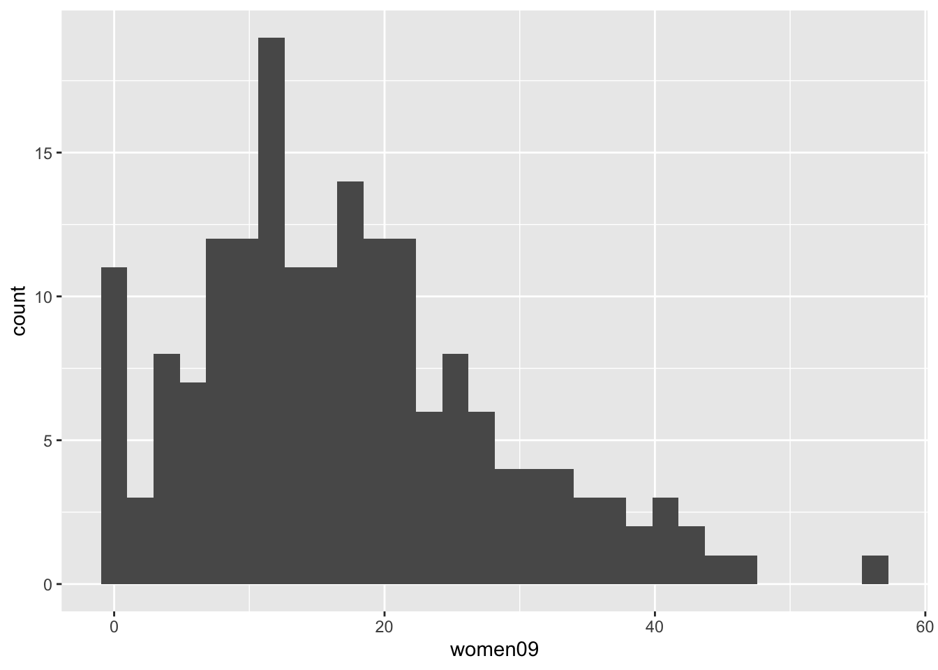
Another way of summarizing the information contained in numerical variables is to visualize the distribution of the variables. Histogram is one of the most commonly used graphical tool to summarize the central tendency and dispersion of numerical variables.
To draw a histogram using the ggplot function, we write:
ggplot(world.data, aes(x = women09)) + geom_histogram()
## `stat_bin()` using `bins = 30`. Pick better value with `binwidth`.

## Warning: Removed 11 rows containing non-finite outside the scale range
## (`stat_bin()`).
ggplot(world.data, aes(x = women09)) + geom_histogram(binwidth = 1)
## Warning: Removed 11 rows containing non-finite outside the scale range
## (`stat_bin()`).
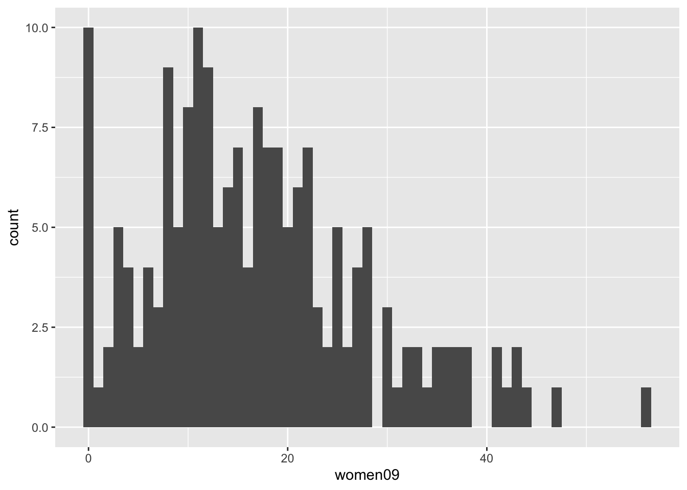
# Notice that we replace x = colony with x = women09
# and geom_bar() with geom_histogram()