Instructions
- Homework assignment is here with all questions commented out.
- Complete all of the coding tasks in the
.qmd file
- Upload your individual exercise to your
GitHub repo by Wed 11:59pm.
- Remember to clean your github repo and sort hw submissions by weeks. Each week should have one folder.
# Preparation -------------------------------------------------------------
rm(list = ls())       # delete everything in the memory
library(ggplot2)      # for graphics
library(Hmisc)        # for rcorr
##
## Attaching package: 'Hmisc'
## The following objects are masked from 'package:base':
##
##     format.pval, units
library(stargazer) # Regression table
##
## Please cite as:
## Hlavac, Marek (2022). stargazer: Well-Formatted Regression and Summary Statistics Tables.
## R package version 5.2.3. https://CRAN.R-project.org/package=stargazer
library(effects) # for effect
## Loading required package: carData
## lattice theme set by effectsTheme()
## See ?effectsTheme for details.
# Read-in the world data
path <- "/Users/howardliu/methodsPol/content/assignment/"
world.data <- read.csv(paste0(path, "world.csv"))


# Task 1 ------------------------------------------------------------------
# Examine the data

#---------------------------------------
# Describe Y
#---------------------------------------

# Numerical summary
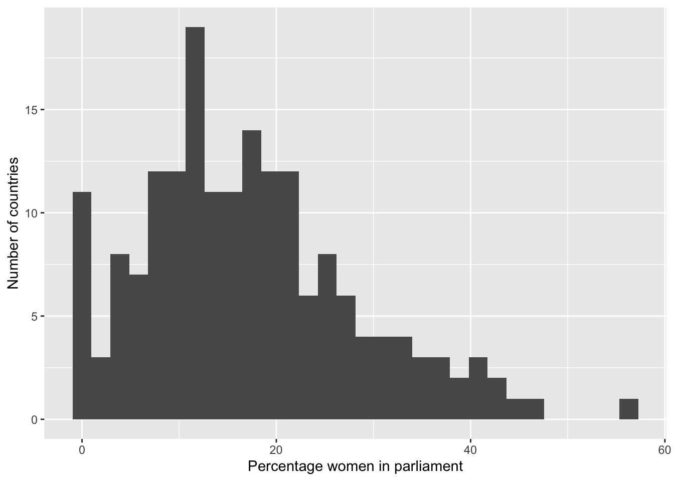
summary(world.data $ women09)
##    Min. 1st Qu.  Median    Mean 3rd Qu.    Max.    NA's
##    0.00    9.70   15.55   17.18   22.95   56.30      11
# Graphical summary
g <- ggplot( world.data, aes( x = women09 ) ) + geom_histogram()
g <- g + ylab("Number of countries") + xlab("Percentage women in parliament")
g
## `stat_bin()` using `bins = 30`. Pick better value `binwidth`.
## Warning: Removed 11 rows containing non-finite outside the scale range
## (`stat_bin()`).

#---------------------------------------
# Describe X: per capita GDP
#---------------------------------------

# Numerical summary
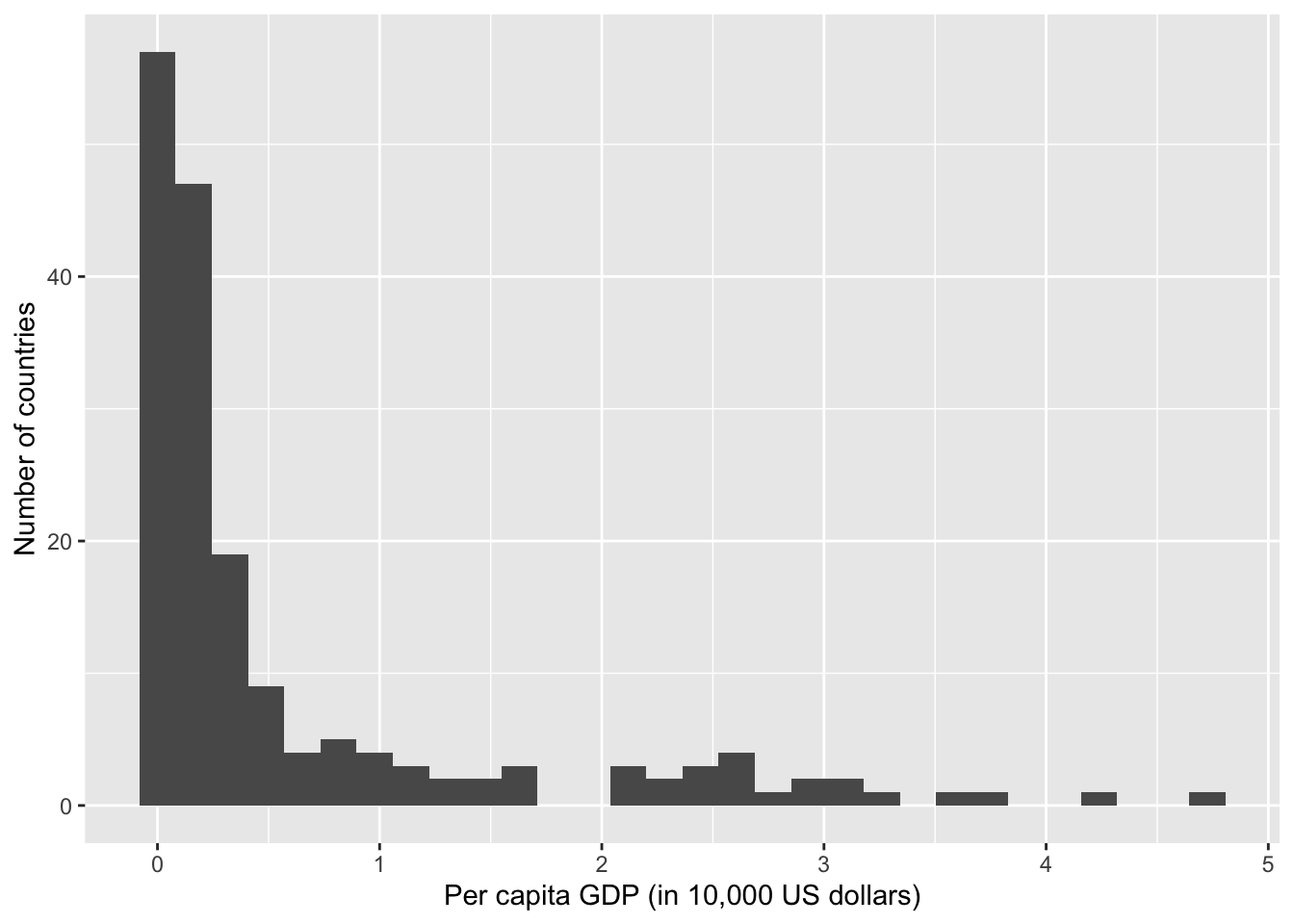
summary(world.data $ gdp_10_thou)
##    Min. 1st Qu.  Median    Mean 3rd Qu.    Max.    NA's
##  0.0090  0.0503  0.1897  0.6018  0.6320  4.7354      14
# Graphical summary
g <- ggplot( world.data, aes( x = gdp_10_thou ) ) + geom_histogram()
g <- g + ylab("Number of countries") + xlab("Per capita GDP (in 10,000 US dollars)")
g
## `stat_bin()` using `bins = 30`. Pick better value `binwidth`.
## Warning: Removed 14 rows containing non-finite outside the scale range
## (`stat_bin()`).

#---------------------------------------
# Describe X-Y
#---------------------------------------
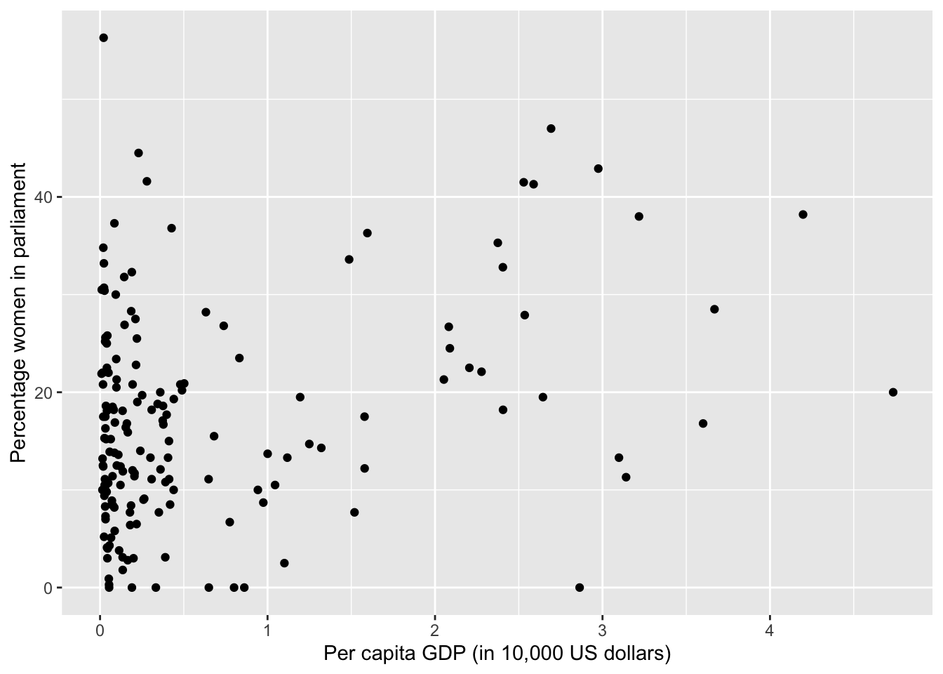
# To describe an X-Y relationship graphically, we draw what's called a
# scatterplot that shows the values of the X variable on the X-axis and
# the values of the Y variable on the Y-axis for all observations.

# To create a scatterplot, we use the geom_point function (because
# each observation is denoted by a point.)

g <- ggplot(world.data, aes( x = gdp_10_thou, y = women09) ) + geom_point()
g <- g + ylab("Percentage women in parliament") + xlab("Per capita GDP (in 10,000 US dollars)")
g
## Warning: Removed 22 rows containing missing values or values outside the scale range
## (`geom_point()`).

# Task 2 ------------------------------------------------------------------
# Omit observations with NAs

women.gdp <- world.data[is.na(world.data $ women09) == FALSE & is.na(world.data $ gdp_10_thou) == FALSE, ]

dim(women.gdp)
## [1] 169 62
# Task 3 ------------------------------------------------------------------
# Calculate test-statistic & p-value

# The test statistic for a bivariate test of two numerical variables is
# (Pearson's) correlation coefficient.

# To calculate correlation coefficient (r), we first need to create a matrix object
# using the as.matrix function.

women.gdp.mat <- as.matrix(women.gdp[ c("gdp_10_thou","women09")])

# Then we use the rcorr function available in the Hmisc package.

rcorr(women.gdp.mat, type = "pearson")
##             gdp_10_thou women09
## gdp_10_thou        1.00    0.31
## women09            0.31    1.00
##
## n= 169
##
##
## P
##             gdp_10_thou women09
## gdp_10_thou              0
## women09      0
# The correlation coefficient is 0.31 with the p-value < 0.001.
# The relationship is positive and highly statistically significant.

# Task 4 ------------------------------------------------------------------
# H0: the effect of gdp_10_thou on women09 is zero.
# Ha: the effect of gdp_10_thou on women09 is positive.


# Task 5 ------------------------------------------------------------------
# Regression

fit.wg <- lm(women09 ~ gdp_10_thou, data = women.gdp)

stargazer(fit.wg, type = "text")
##
## ===============================================
##                         Dependent variable:
##                     ---------------------------
##                               women09
## -----------------------------------------------
## gdp_10_thou                  3.457***
##                               (0.835)
##
## Constant                     14.843***
##                               (0.954)
##
## -----------------------------------------------
## Observations                    169
## R2                             0.093
## Adjusted R2                    0.088
## Residual Std. Error      10.379 (df = 167)
## F Statistic           17.139*** (df = 1; 167)
## ===============================================
## Note:               *p<0.1; **p<0.05; ***p<0.01
# (a)
# Regression equation: women09 = 14.843 + 3.457 * gdp_10_thou

# (b)
# Positive

# (c)
# An increase in per capita GDP (gdp_10_thou) by 10000 dollars will lead to an increase
# in female representation by 3.457 percentage points.
# An increase in per capita GDP (gdp_10_thou) by 1000 dollars will lead to an increase
# in female representation by 0.3457 percentage points.

# (d)
# The estimated coefficient for gdp_10_thou is highly statistically significant.
# We can reject the null hypothesis at 1% significance level.


# Task 6 ------------------------------------------------------------------
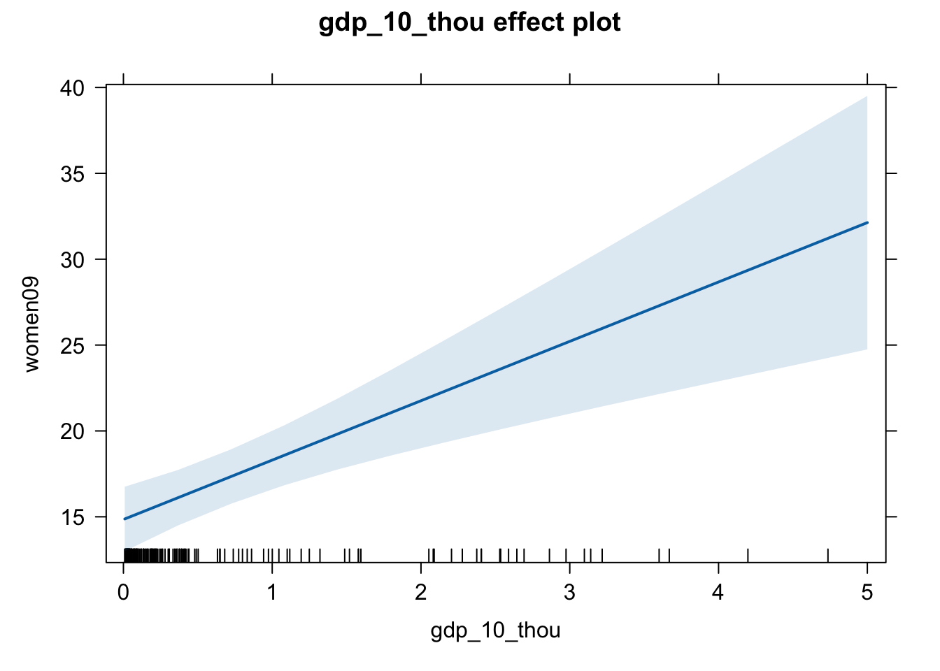
eff.wg <- effect(term = "gdp_10_thou", mod = fit.wg)

plot(eff.wg)

# Task 7 ------------------------------------------------------------------

stargazer(fit.wg, type = "text")
##
## ===============================================
##                         Dependent variable:
##                     ---------------------------
##                               women09
## -----------------------------------------------
## gdp_10_thou                  3.457***
##                               (0.835)
##
## Constant                     14.843***
##                               (0.954)
##
## -----------------------------------------------
## Observations                    169
## R2                             0.093
## Adjusted R2                    0.088
## Residual Std. Error      10.379 (df = 167)
## F Statistic           17.139*** (df = 1; 167)
## ===============================================
## Note:               *p<0.1; **p<0.05; ***p<0.01
# (a)
# The R-squared is 0.093, which means that about 9% of the total variation in
# Female Representation is explained by per capita GDP.

# Many factors could potentially influence the variation in female representation
# across countries, and economic development appears to be one of them.
# R-squred of 9 % seems rather small, and it implies that either our model ignores
# some other important determinants, or the variation in female representation
# is quite random.


# (b)
# The Residual Std. Error is 10.379. That is, our predictions are off by about
# 10 percentage points, on average. I would say that this is rather big.
# Again, this implies that either our model ignores some other important
# determinants, or the variation in female representation is quite random.


# Task 8 ------------------------------------------------------------------
# Predicted values
women.gdp $ y.hat <- predict(fit.wg)

# Values for Rwanda
women.gdp[ women.gdp $ country == "Rwanda", c("women09", "y.hat") ]
##     women09    y.hat
## 142    56.3 14.91632
# The predicted value of Female Representation for Rwanda is 14.91%, whereas
# the actual value is 56.3%. I would say that our prediction is very, very far off.


# Task 9 ------------------------------------------------------------------
# Do the analyses for PR and non-PR countries seperately to control for
# electoral system "manually".

# Re-label the PR variable
women.gdp $ pr <- factor(women.gdp $ pr_sys, levels = c("No", "Yes"), labels = c("Non-PR", "PR"))

# Make sure it worked
table(women.gdp $ pr_sys, women.gdp $ pr)
##
##       Non-PR  PR
##   No     106   0
##   Yes      0  63
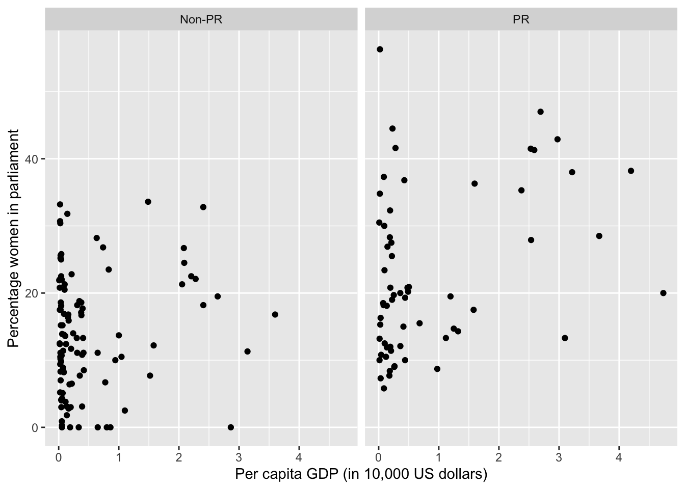
# Examine the X-Y relationship graphically
g <- ggplot(women.gdp, aes( x = gdp_10_thou, y = women09) ) + geom_point()
g <- g + ylab("Percentage women in parliament") + xlab("Per capita GDP (in 10,000 US dollars)")
g <- g + facet_grid( ~ pr)
g

# Create data sets for PR and non-PR
women.gdp.pr <- women.gdp[women.gdp $ pr == "PR", ]
women.gdp.mj <- women.gdp[women.gdp $ pr == "Non-PR", ]

# Separate regression models for PR and non-PR

fit.wg.pr <- lm(women09 ~ gdp_10_thou, data = women.gdp.pr)
fit.wg.mj <- lm(women09 ~ gdp_10_thou, data = women.gdp.mj)

stargazer(fit.wg.pr, type = "text")
##
## ===============================================
##                         Dependent variable:
##                     ---------------------------
##                               women09
## -----------------------------------------------
## gdp_10_thou                  3.641***
##                               (1.218)
##
## Constant                     19.375***
##                               (1.748)
##
## -----------------------------------------------
## Observations                    63
## R2                             0.128
## Adjusted R2                    0.113
## Residual Std. Error      11.254 (df = 61)
## F Statistic            8.935*** (df = 1; 61)
## ===============================================
## Note:               *p<0.1; **p<0.05; ***p<0.01
stargazer(fit.wg.mj, type = "text")
##
## ===============================================
##                         Dependent variable:
##                     ---------------------------
##                               women09
## -----------------------------------------------
## gdp_10_thou                    1.655
##                               (1.081)
##
## Constant                     12.956***
##                               (1.001)
##
## -----------------------------------------------
## Observations                    106
## R2                             0.022
## Adjusted R2                    0.013
## Residual Std. Error      8.685 (df = 104)
## F Statistic             2.343 (df = 1; 104)
## ===============================================
## Note:               *p<0.1; **p<0.05; ***p<0.01
# Alternatively, we can have one table that summarizes two (or more)
# regression models, as follows:

stargazer(fit.wg.pr, fit.wg.mj, type = "text")
##
## =============================================================
##                                Dependent variable:
##                     -----------------------------------------
##                                      women09
##                              (1)                  (2)
## -------------------------------------------------------------
## gdp_10_thou               3.641***               1.655
##                            (1.218)              (1.081)
##
## Constant                  19.375***            12.956***
##                            (1.748)              (1.001)
##
## -------------------------------------------------------------
## Observations                 63                   106
## R2                          0.128                0.022
## Adjusted R2                 0.113                0.013
## Residual Std. Error   11.254 (df = 61)     8.685 (df = 104)
## F Statistic         8.935*** (df = 1; 61) 2.343 (df = 1; 104)
## =============================================================
## Note:                             *p<0.1; **p<0.05; ***p<0.01
# Task 10 -----------------------------------------------------------------
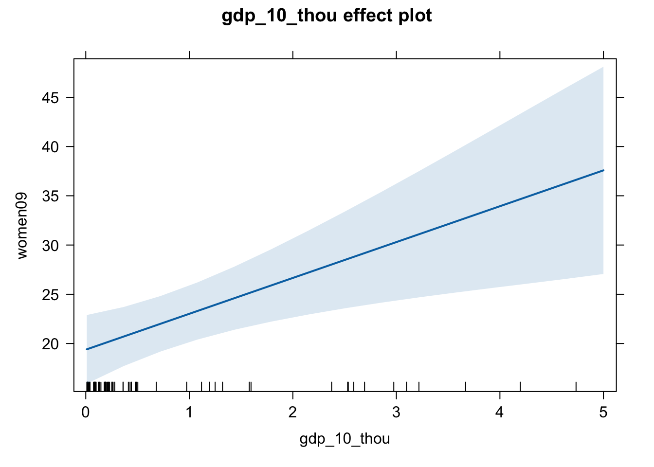
# The estimated effect of gdp_10_thou for PR countries.

# From the stargazer table above, we can see that the estimated effect of
# gdp_10_thou on women09 is positive (3.641) and statistically significant
# for PR countries (p < 0.01).

eff.wg.pr <- effect(term = "gdp_10_thou", mod = fit.wg.pr)
plot(eff.wg.pr)

# Task 11 -----------------------------------------------------------------
# The estimated effect of gdp_10_thou for non-PR countries.

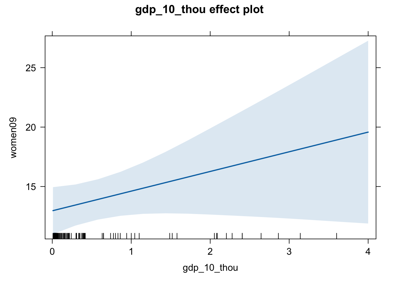
# From the stargazer table above, we can see that the estimated effect of
# gdp_10_thou on women09 is positive (1.655) but not statistically significant.
# That is, we cannot reject the null hypothesis that the effect is zero.

eff.wg.mj <- effect(term = "gdp_10_thou", mod = fit.wg.mj)
plot(eff.wg.mj)

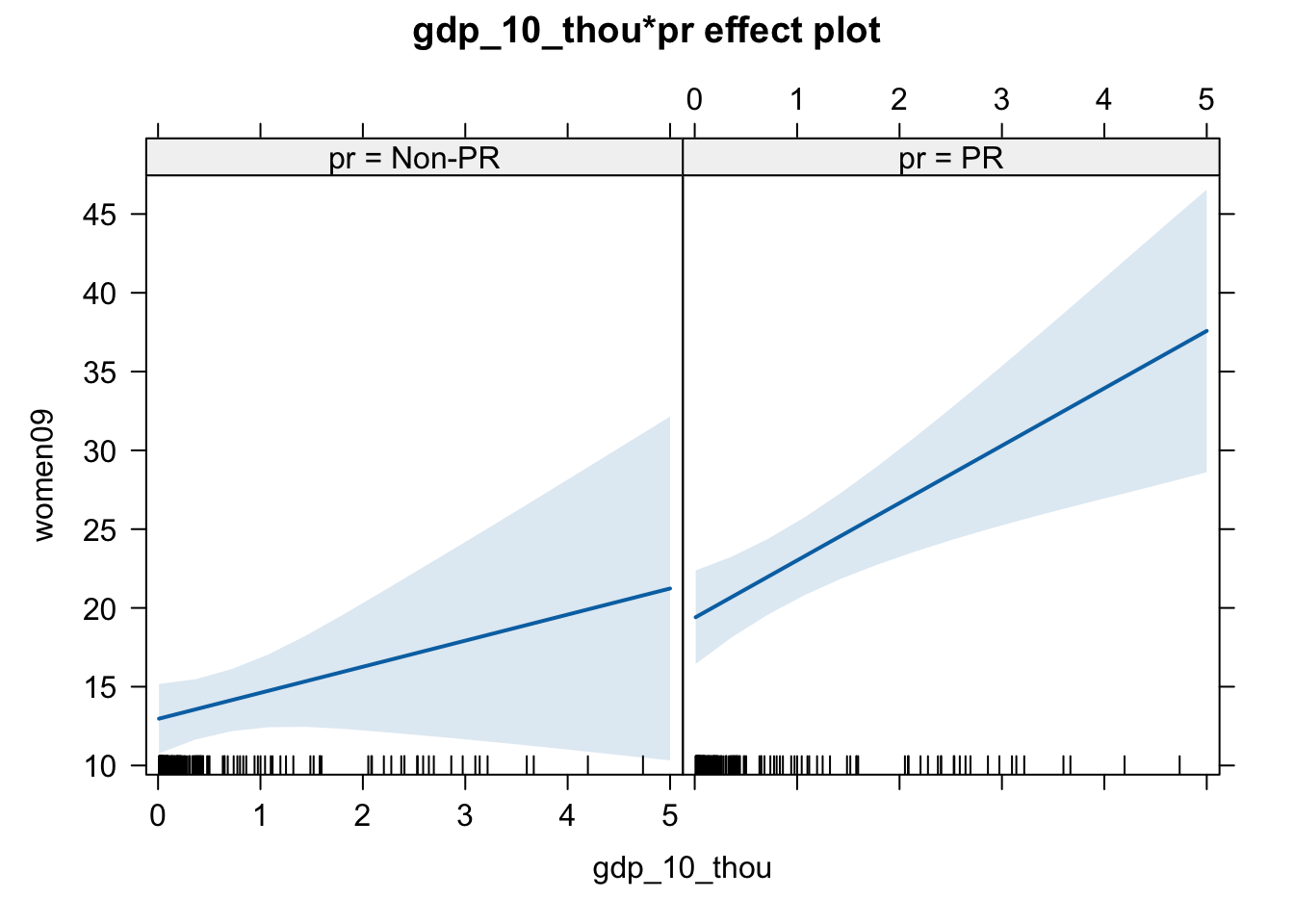
# Advanced: If you want to create a graph that shows the estimated effects
# of X on Y for two different scenarios (PR and non-PR), we can do the following.
# We will talk a lot more about this type of analyses in the Spring term.

fit.i <- lm(women09 ~ gdp_10_thou + pr + gdp_10_thou:pr, data = women.gdp)
eff.i <- effect(term = "gdp_10_thou:pr", mod = fit.i)
plot(eff.i)

# Task 12 -----------------------------------------------------------------
# Predicted values.

women.gdp.pr $ y.hat <- predict(fit.wg.pr)

# Values for Rwanda
women.gdp.pr[ women.gdp.pr $ country == "Rwanda", c("women09", "y.hat") ]
##     women09    y.hat
## 142    56.3 19.45267
