Data management (answers)
Instructions
- Homework assignment is here with all questions commented out.
- Complete all of the coding tasks in the
.qmdfile - Upload your individual exercise to your
GitHubrepo by Wed 11:59pm. - Remember to clean your github repo and sort hw submissions by weeks. Each week should have one folder.
- You can find my code here
1. Exploring a data set
We have learned several functions to explore a data set, including
library(ggplot2)
library(tidyverse)
world.data <- read.csv("world.csv")
table( world.data $ democ_regime )
##
##  No Yes
##  75 114
dim(world.data)
## [1] 191 62
head(world.data)
##             country       colony confidence decentralization dem_other
## 1       Afghanistan           UK         NA               NA      10.5
## 2           Albania Soviet Union   49.33593             0.74      63.0
## 3           Algeria       France   52.05573               NA      40.8
## 4           Andorra        Spain         NA               NA     100.0
## 5            Angola     Portugal         NA               NA      40.8
## 6 Antigua & Barbuda           UK         NA               NA      87.5
##   dem_other5 democ_regime    district_size3 durable effectiveness      enpp_3
## 1        10%           No     single member       4      13.71158
## 2 Approx 60%          Yes                         3      35.46099 1-3 parties
## 3 Approx 40%           No 6 or more members       5      32.62411
## 4       100%          Yes                        NA      78.72340
## 5 Approx 40%           No                         3      19.14894
## 6 Approx 90%          Yes     single member      NA      59.81088 1-3 parties
##           eu fhrate04_rev fhrate08_rev frac_eth frac_eth3 free_business
## 1 Not member          2.5            3   0.7693      High            NA
## 2 Not member            5            8   0.2204       Low          68.0
## 3 Not member          2.5            3   0.3394    Medium          71.2
## 4 Not member    Most free           12   0.7139      High            NA
## 5 Not member          2.5            3   0.7867      High          43.4
## 6 Not member            6           10   0.1643       Low            NA
##   free_corrupt free_finance free_fiscal free_govspend free_invest free_labor
## 1           NA           NA          NA            NA          NA         NA
## 2           34           70        92.6          74.2          70       52.1
## 3           32           30        83.5          73.4          45       56.4
## 4           NA           NA          NA            NA          NA         NA
## 5           19           40        85.1          62.8          35       45.2
## 6           NA           NA          NA            NA          NA         NA
##   free_monetary free_overall free_property free_trade gdp08 gdp_10_thou
## 1            NA           NA            NA         NA  30.6          NA
## 2          78.7         66.0            35       85.8  24.3      0.1535
## 3          77.2         56.9            30       70.7 276.0      0.1785
## 4            NA           NA            NA         NA    NA          NA
## 5          62.6         48.4            20       70.4 106.3      0.0857
## 6            NA           NA            NA         NA    NA      1.0449
##   gdp_cap2 gdp_cap3 gdppcap08 gender_equal3 gini04 gini08   hi_gdp indy
## 1                          NA                   NA     NA          1919
## 2      Low   Middle      7715                 28.2   31.1  Low GDP 1991
## 3      Low   Middle      8033                 35.3   35.3  Low GDP 1962
## 4                          NA                   NA     NA          1278
## 5      Low   Middle      5899                   NA     NA  Low GDP 1975
## 6     High     High        NA                   NA     NA High GDP 1981
##         oecd  old2006  old2003     pmat12_3    pop03 pop08    pop08_3
## 1 Not member       NA       NA                    NA  27.4 >=16.8 mil
## 2 Not member 8.479821 7.278363 Low post-mat  3169064   3.1  <=4.3 mil
## 3 Not member 4.578136 4.045199              31832610  34.4 >=16.8 mil
## 4 Not member       NA       NA                 66000    NA
## 5 Not member 2.450295 2.930542              13522110  18.0 >=16.8 mil
## 6 Not member       NA 8.186610                 78580    NA
##            popcat3 pr_sys protact3        regime_type3      region sources
## 1 Moderate (1-29m)     No                 Dictatorship Middle East      NA
## 2 Moderate (1-29m)     No Moderate Parliamentary democ  C&E Europe      NA
## 3 Moderate (1-29m)    Yes                 Dictatorship      Africa      NA
## 4 Small (under 1m)     No          Parliamentary democ   W. Europe      NA
## 5 Moderate (1-29m)    Yes                 Dictatorship      Africa      NA
## 6 Small (under 1m)     No          Parliamentary democ  S. America      NA
##          typerel unions urban03 urban06 vi_rel3 votevap00s women05 women09
## 1         Muslim     NA      NA   23.28                 NA      NA    27.7
## 2         Muslim     NA 44.2390   46.14  20-50%      59.56     6.4    16.4
## 3         Muslim     NA 58.8302   63.94    >50%         NA      NA     7.7
## 4 Roman Catholic     NA 91.7404   90.28              20.95    14.3    35.7
## 5 Roman Catholic     NA 36.1806   53.96                 NA      NA    37.3
## 6     Protestant     NA 37.7566   39.60              76.34    10.5    10.5
##   womyear       womyear2  yng2003  young06
## 1      NA                      NA       NA
## 2    1920 1944 or before 27.34834 26.35428
## 3    1962     After 1944 33.91887 28.94154
## 4    1973     After 1944       NA       NA
## 5    1975     After 1944 47.62524 46.32196
## 6    1951     After 1944 20.66509       NA
tail(world.data)
##                 country       colony confidence decentralization dem_other
## 186             Vietnam       France   99.86241               NA      58.3
## 187       Western Samoa        Other         NA               NA      58.3
## 188               Yemen           UK         NA               NA      10.5
## 189 Serbia & Montenegro Soviet Union   31.64857               NA      63.0
## 190              Zambia           UK         NA               NA      40.8
## 191            Zimbabwe           UK   60.01903             0.87      40.8
##     dem_other5 democ_regime  district_size3 durable effectiveness      enpp_3
## 186 Approx 60%           No >1 to 5 members      46      40.18912
## 187 Approx 60%           No   single member      NA      52.00946
## 188        10%           No   single member       7      26.00473
## 189 Approx 60%           No >1 to 5 members       0      29.31442
## 190 Approx 40%          Yes   single member       4      24.58629 1-3 parties
## 191 Approx 40%           No   single member      13      27.65957
##             eu fhrate04_rev fhrate08_rev frac_eth frac_eth3 free_business
## 186 Not member          1.5            2   0.2383       Low          60.7
## 187 Not member            6           10   0.1376       Low          73.2
## 188 Not member            3            4       NA                    74.4
## 189 Not member          5.5            9   0.5736    Medium            NA
## 190 Not member            4            8   0.7808      High          66.4
## 191 Not member          1.5            1   0.3874    Medium          30.0
##     free_corrupt free_finance free_fiscal free_govspend free_invest free_labor
## 186           27           30        76.1          73.4          20       68.4
## 187           44           30        79.6          67.5          30       80.8
## 188           23           30        83.2          51.3          45       65.4
## 189           NA           NA          NA            NA          NA         NA
## 190           28           50        72.4          82.6          50       57.0
## 191           18           10        58.4            NA          NA       48.2
##     free_monetary free_overall free_property free_trade gdp08 gdp_10_thou
## 186          58.1         49.8            15       68.9 240.1      0.0436
## 187          73.8         60.4            55       70.0   0.8      0.1484
## 188          65.1         54.4            30       76.1  55.3      0.0537
## 189            NA           NA            NA         NA    NA      0.1922
## 190          63.3         58.0            30       79.9  17.1      0.0361
## 191            NA         21.4             5       44.8   2.2      0.0639
##     gdp_cap2 gdp_cap3 gdppcap08 gender_equal3 gini04 gini08   hi_gdp indy
## 186      Low      Low      2785                 36.1   34.4  Low GDP 1962
## 187      Low   Middle      4485                   NA     NA  Low GDP 1990
## 188      Low      Low      2400           Low   33.4   33.4  Low GDP 1991
## 189     High   Middle        NA                   NA     NA High GDP 1964
## 190      Low      Low      1356                 52.6   50.8  Low GDP 1980
## 191      Low      Low       188                 56.8   50.1  Low GDP 1980
##           oecd   old2006   old2003     pmat12_3    pop03 pop08      pop08_3
## 186 Not member  5.437487  5.261546              81314240  86.2   >=16.8 mil
## 187 Not member  4.595193  4.978562                178000   0.2    <=4.3 mil
## 188 Not member  2.284142  2.622207              19173160  23.1   >=16.8 mil
## 189 Not member 14.114708 14.008000 Low post-mat  8104000    NA
## 190 Not member  3.032360  2.693117              10402960  12.6 4.4-16.4 mil
## 191 Not member  3.711219  3.101562              13101750  11.7 4.4-16.4 mil
##              popcat3 pr_sys protact3       regime_type3       region sources
## 186     Large (30m+)     No                Dictatorship Asia-Pacific      NA
## 187 Small (under 1m)     No                Dictatorship Asia-Pacific      NA
## 188 Moderate (1-29m)     No                Dictatorship  Middle East      NA
## 189 Moderate (1-29m)     No      Low       Dictatorship   C&E Europe      NA
## 190 Moderate (1-29m)     No          Presidential democ       Africa      NA
## 191 Moderate (1-29m)     No                Dictatorship       Africa      NA
##        typerel unions urban03 urban06 vi_rel3 votevap00s women05 women09
## 186    eastern     NA 25.4076   26.88    <20%         NA      NA    25.8
## 187 Protestant     NA 22.8014   22.60              76.62      NA      NA
## 188     Muslim     NA 25.6836   27.72                 NA      NA     0.3
## 189   Orthodox     NA 52.0384   52.44  20-50%         NA      NA      NA
## 190      other   12.5 40.3128   35.14              55.74    12.7    15.2
## 191 Protestant   13.9 37.4674   36.38    >50%         NA      NA    15.2
##     womyear   womyear2  yng2003  young06
## 186    1946 After 1944 30.62024 28.78953
## 187    1990 After 1944 35.46627 40.41566
## 188    1967 After 1944 45.24762 45.99981
## 189    1946 After 1944 19.59660 18.03825
## 190    1962 After 1944 46.82837 45.63621
## 191    1957 After 1944 43.43543 39.46990
There are some other functions we can use. For example, the names function tells us the names of all the variables included in a data frame object.
names(world.data)
##  [1] "country"          "colony"           "confidence"       "decentralization"
##  [5] "dem_other"        "dem_other5"       "democ_regime"     "district_size3"
##  [9] "durable"          "effectiveness"    "enpp_3"           "eu"
## [13] "fhrate04_rev"     "fhrate08_rev"     "frac_eth"         "frac_eth3"
## [17] "free_business"    "free_corrupt"     "free_finance"     "free_fiscal"
## [21] "free_govspend"    "free_invest"      "free_labor"       "free_monetary"
## [25] "free_overall"     "free_property"    "free_trade"       "gdp08"
## [29] "gdp_10_thou"      "gdp_cap2"         "gdp_cap3"         "gdppcap08"
## [33] "gender_equal3"    "gini04"           "gini08"           "hi_gdp"
## [37] "indy"             "oecd"             "old2006"          "old2003"
## [41] "pmat12_3"         "pop03"            "pop08"            "pop08_3"
## [45] "popcat3"          "pr_sys"           "protact3"         "regime_type3"
## [49] "region"           "sources"          "typerel"          "unions"
## [53] "urban03"          "urban06"          "vi_rel3"          "votevap00s"
## [57] "women05"          "women09"          "womyear"          "womyear2"
## [61] "yng2003"          "young06"
The colnames function gives us the same results as well.
colnames(world.data)
##  [1] "country"          "colony"           "confidence"       "decentralization"
##  [5] "dem_other"        "dem_other5"       "democ_regime"     "district_size3"
##  [9] "durable"          "effectiveness"    "enpp_3"           "eu"
## [13] "fhrate04_rev"     "fhrate08_rev"     "frac_eth"         "frac_eth3"
## [17] "free_business"    "free_corrupt"     "free_finance"     "free_fiscal"
## [21] "free_govspend"    "free_invest"      "free_labor"       "free_monetary"
## [25] "free_overall"     "free_property"    "free_trade"       "gdp08"
## [29] "gdp_10_thou"      "gdp_cap2"         "gdp_cap3"         "gdppcap08"
## [33] "gender_equal3"    "gini04"           "gini08"           "hi_gdp"
## [37] "indy"             "oecd"             "old2006"          "old2003"
## [41] "pmat12_3"         "pop03"            "pop08"            "pop08_3"
## [45] "popcat3"          "pr_sys"           "protact3"         "regime_type3"
## [49] "region"           "sources"          "typerel"          "unions"
## [53] "urban03"          "urban06"          "vi_rel3"          "votevap00s"
## [57] "women05"          "women09"          "womyear"          "womyear2"
## [61] "yng2003"          "young06"
We can also apply the summary function without specifying variable names. Then, R will provide the summary of ALL the variables included in a data frame object.
summary(world.data)
##    country             colony            confidence      decentralization
##  Length:191         Length:191         Min.   : 0.5167   Min.   :0.380
##  Class :character   Class :character   1st Qu.:38.3669   1st Qu.:1.225
##  Mode  :character   Mode  :character   Median :49.1978   Median :1.510
##                                        Mean   :47.9704   Mean   :1.516
##                                        3rd Qu.:59.2929   3rd Qu.:1.800
##                                        Max.   :99.8624   Max.   :2.450
##                                        NA's   :120       NA's   :124
##    dem_other       dem_other5        democ_regime       district_size3
##  Min.   : 10.50   Length:191         Length:191         Length:191
##  1st Qu.: 40.80   Class :character   Class :character   Class :character
##  Median : 58.30   Mode  :character   Mode  :character   Mode  :character
##  Mean   : 60.51
##  3rd Qu.: 87.50
##  Max.   :100.00
##
##     durable       effectiveness       enpp_3               eu
##  Min.   :  0.00   Min.   :  0.00   Length:191         Length:191
##  1st Qu.:  4.00   1st Qu.: 28.19   Class :character   Class :character
##  Median :  9.00   Median : 40.31   Mode  :character   Mode  :character
##  Mean   : 22.49   Mean   : 45.77
##  3rd Qu.: 31.25   3rd Qu.: 62.77
##  Max.   :191.00   Max.   :100.00
##  NA's   :31       NA's   :5
##  fhrate04_rev        fhrate08_rev       frac_eth       frac_eth3
##  Length:191         Min.   : 0.000   Min.   :0.0000   Length:191
##  Class :character   1st Qu.: 4.000   1st Qu.:0.1997   Class :character
##  Mode  :character   Median : 8.000   Median :0.4343   Mode  :character
##                     Mean   : 7.553   Mean   :0.4394
##                     3rd Qu.:11.250   3rd Qu.:0.6611
##                     Max.   :12.000   Max.   :0.9302
##                     NA's   :3        NA's   :3
##  free_business    free_corrupt    free_finance    free_fiscal
##  Min.   :10.00   Min.   : 5.00   Min.   :10.00   Min.   :35.90
##  1st Qu.:55.70   1st Qu.:26.00   1st Qu.:30.00   1st Qu.:68.20
##  Median :65.80   Median :34.00   Median :50.00   Median :77.50
##  Mean   :64.92   Mean   :40.42   Mean   :48.61   Mean   :75.62
##  3rd Qu.:76.60   3rd Qu.:51.75   3rd Qu.:60.00   3rd Qu.:84.00
##  Max.   :99.90   Max.   :93.00   Max.   :90.00   Max.   :99.90
##  NA's   :18      NA's   :17      NA's   :18      NA's   :18
##  free_govspend    free_invest      free_labor    free_monetary
##  Min.   : 6.90   Min.   : 5.00   Min.   :20.00   Min.   :46.50
##  1st Qu.:54.95   1st Qu.:35.00   1st Qu.:50.10   1st Qu.:66.85
##  Median :73.40   Median :50.00   Median :60.80   Median :71.90
##  Mean   :67.59   Mean   :50.75   Mean   :62.08   Mean   :71.30
##  3rd Qu.:83.25   3rd Qu.:70.00   3rd Qu.:75.90   3rd Qu.:76.55
##  Max.   :98.40   Max.   :95.00   Max.   :98.90   Max.   :88.80
##  NA's   :24      NA's   :24      NA's   :18      NA's   :19
##   free_overall   free_property    free_trade        gdp08
##  Min.   : 1.00   Min.   : 5.0   Min.   :31.90   Min.   :    0.2
##  1st Qu.:51.35   1st Qu.:30.0   1st Qu.:67.20   1st Qu.:   11.9
##  Median :59.30   Median :40.0   Median :75.90   Median :   41.7
##  Mean   :59.18   Mean   :43.9   Mean   :74.37   Mean   :  390.4
##  3rd Qu.:67.30   3rd Qu.:60.0   3rd Qu.:85.00   3rd Qu.:  242.4
##  Max.   :86.10   Max.   :95.0   Max.   :90.00   Max.   :14200.0
##  NA's   :17      NA's   :18     NA's   :18      NA's   :14
##   gdp_10_thou       gdp_cap2           gdp_cap3           gdppcap08
##  Min.   :0.0090   Length:191         Length:191         Min.   :   188
##  1st Qu.:0.0503   Class :character   Class :character   1st Qu.:  2308
##  Median :0.1897   Mode  :character   Mode  :character   Median :  7703
##  Mean   :0.6018                                         Mean   : 13828
##  3rd Qu.:0.6320                                         3rd Qu.: 19996
##  Max.   :4.7354                                         Max.   :118040
##  NA's   :14                                             NA's   :16
##  gender_equal3          gini04          gini08         hi_gdp
##  Length:191         Min.   :24.40   Min.   :24.70   Length:191
##  Class :character   1st Qu.:32.42   1st Qu.:33.55   Class :character
##  Mode  :character   Median :37.95   Median :39.20   Mode  :character
##                     Mean   :40.14   Mean   :40.74
##                     3rd Qu.:46.88   3rd Qu.:47.10
##                     Max.   :70.70   Max.   :74.30
##                     NA's   :65      NA's   :64
##       indy          oecd              old2006          old2003
##  Min.   : 301   Length:191         Min.   : 1.076   Min.   : 1.846
##  1st Qu.:1915   Class :character   1st Qu.: 3.375   1st Qu.: 3.173
##  Median :1960   Mode  :character   Median : 4.924   Median : 4.865
##  Mean   :1891                      Mean   : 7.300   Mean   : 6.979
##  3rd Qu.:1977                      3rd Qu.:11.210   3rd Qu.:10.656
##  Max.   :1994                      Max.   :20.232   Max.   :18.997
##  NA's   :3                         NA's   :17       NA's   :10
##    pmat12_3             pop03               pop08           pop08_3
##  Length:191         Min.   :2.000e+04   Min.   :   0.00   Length:191
##  Class :character   1st Qu.:1.758e+06   1st Qu.:   2.70   Class :character
##  Mode  :character   Median :6.720e+06   Median :   8.30   Mode  :character
##                     Mean   :3.318e+07   Mean   :  36.95
##                     3rd Qu.:2.121e+07   3rd Qu.:  24.60
##                     Max.   :1.288e+09   Max.   :1300.00
##                     NA's   :4           NA's   :14
##    popcat3             pr_sys            protact3         regime_type3
##  Length:191         Length:191         Length:191         Length:191
##  Class :character   Class :character   Class :character   Class :character
##  Mode  :character   Mode  :character   Mode  :character   Mode  :character
##
##
##
##
##     region          sources          typerel              unions
##  Length:191         Mode:logical   Length:191         Min.   : 2.00
##  Class :character   NA's:191       Class :character   1st Qu.:11.45
##  Mode  :character                  Mode  :character   Median :19.10
##                                                       Mean   :24.74
##                                                       3rd Qu.:30.80
##                                                       Max.   :96.10
##                                                       NA's   :100
##     urban03           urban06         vi_rel3            votevap00s
##  Min.   :  6.556   Min.   : 10.32   Length:191         Min.   :18.29
##  1st Qu.: 36.413   1st Qu.: 35.49   Class :character   1st Qu.:54.58
##  Median : 57.491   Median : 56.76   Mode  :character   Median :65.12
##  Mean   : 55.620   Mean   : 54.55                      Mean   :65.08
##  3rd Qu.: 73.830   3rd Qu.: 72.75                      3rd Qu.:77.66
##  Max.   :100.000   Max.   :100.00                      Max.   :98.39
##  NA's   :5         NA's   :4                           NA's   :92
##     women05         women09         womyear       womyear2
##  Min.   : 0.00   Min.   : 0.00   Min.   :1893   Length:191
##  1st Qu.: 8.25   1st Qu.: 9.70   1st Qu.:1931   Class :character
##  Median :13.00   Median :15.55   Median :1949   Mode  :character
##  Mean   :15.38   Mean   :17.18   Mean   :1947
##  3rd Qu.:20.45   3rd Qu.:22.95   3rd Qu.:1960
##  Max.   :45.30   Max.   :56.30   Max.   :1990
##  NA's   :80      NA's   :11      NA's   :16
##     yng2003         young06
##  Min.   :14.02   Min.   :13.50
##  1st Qu.:21.31   1st Qu.:19.53
##  Median :31.95   Median :30.65
##  Mean   :31.41   Mean   :30.45
##  3rd Qu.:41.30   3rd Qu.:39.72
##  Max.   :49.77   Max.   :50.50
##  NA's   :10      NA's   :17
The str() function tells us the structure of a data frame object, meaning that it tells us which variables are factor, which ones are numerical, which ones are logical, etc.
str(world.data)
## 'data.frame':	191 obs. of  62 variables:
##  $ country         : chr  "Afghanistan" "Albania" "Algeria" "Andorra" ...
##  $ colony          : chr  "UK" "Soviet Union" "France" "Spain" ...
##  $ confidence      : num  NA 49.3 52.1 NA NA ...
##  $ decentralization: num  NA 0.74 NA NA NA NA 2.4 NA 1.74 1.81 ...
##  $ dem_other       : num  10.5 63 40.8 100 40.8 87.5 87.5 63 58.3 100 ...
##  $ dem_other5      : chr  "10%" "Approx 60%" "Approx 40%" "100%" ...
##  $ democ_regime    : chr  "No" "Yes" "No" "Yes" ...
##  $ district_size3  : chr  "single member" "" "6 or more members" "" ...
##  $ durable         : int  4 3 5 NA 3 NA 17 2 99 54 ...
##  $ effectiveness   : num  13.7 35.5 32.6 78.7 19.1 ...
##  $ enpp_3          : chr  "" "1-3 parties" "" "" ...
##  $ eu              : chr  "Not member" "Not member" "Not member" "Not member" ...
##  $ fhrate04_rev    : chr  "2.5" "5" "2.5" "Most free" ...
##  $ fhrate08_rev    : int  3 8 3 12 3 10 10 4 12 12 ...
##  $ frac_eth        : num  0.769 0.22 0.339 0.714 0.787 ...
##  $ frac_eth3       : chr  "High" "Low" "Medium" "High" ...
##  $ free_business   : num  NA 68 71.2 NA 43.4 NA 62.1 83.4 90.3 73.6 ...
##  $ free_corrupt    : int  NA 34 32 NA 19 NA 29 29 87 81 ...
##  $ free_finance    : int  NA 70 30 NA 40 NA 30 70 90 70 ...
##  $ free_fiscal     : num  NA 92.6 83.5 NA 85.1 NA 69.5 89.3 61.4 51.2 ...
##  $ free_govspend   : num  NA 74.2 73.4 NA 62.8 NA 75.6 90.9 64.9 28.8 ...
##  $ free_invest     : int  NA 70 45 NA 35 NA 45 75 80 75 ...
##  $ free_labor      : num  NA 52.1 56.4 NA 45.2 NA 50.1 70.6 94.9 79.1 ...
##  $ free_monetary   : num  NA 78.7 77.2 NA 62.6 NA 61.2 72.9 82.7 79.3 ...
##  $ free_overall    : num  NA 66 56.9 NA 48.4 NA 51.2 69.2 82.6 71.6 ...
##  $ free_property   : int  NA 35 30 NA 20 NA 20 30 90 90 ...
##  $ free_trade      : num  NA 85.8 70.7 NA 70.4 NA 69.5 80.5 85.1 87.5 ...
##  $ gdp08           : num  30.6 24.3 276 NA 106.3 ...
##  $ gdp_10_thou     : num  NA 0.1535 0.1785 NA 0.0857 ...
##  $ gdp_cap2        : chr  "" "Low" "Low" "" ...
##  $ gdp_cap3        : chr  "" "Middle" "Middle" "" ...
##  $ gdppcap08       : int  NA 7715 8033 NA 5899 NA 14333 6070 35677 38152 ...
##  $ gender_equal3   : chr  "" "" "" "" ...
##  $ gini04          : num  NA 28.2 35.3 NA NA NA 52.2 37.9 35.2 30 ...
##  $ gini08          : num  NA 31.1 35.3 NA NA NA 51.3 33.8 35.2 29.1 ...
##  $ hi_gdp          : chr  "" "Low GDP" "Low GDP" "" ...
##  $ indy            : int  1919 1991 1962 1278 1975 1981 1816 1991 1901 1156 ...
##  $ oecd            : chr  "Not member" "Not member" "Not member" "Not member" ...
##  $ old2006         : num  NA 8.48 4.58 NA 2.45 ...
##  $ old2003         : num  NA 7.28 4.05 NA 2.93 ...
##  $ pmat12_3        : chr  "" "Low post-mat" "" "" ...
##  $ pop03           : num  NA 3169064 31832610 66000 13522110 ...
##  $ pop08           : num  27.4 3.1 34.4 NA 18 NA 39.9 3.1 21 8.3 ...
##  $ pop08_3         : chr  ">=16.8 mil" "<=4.3 mil" ">=16.8 mil" "" ...
##  $ popcat3         : chr  "Moderate (1-29m)" "Moderate (1-29m)" "Moderate (1-29m)" "Small (under 1m)" ...
##  $ pr_sys          : chr  "No" "No" "Yes" "No" ...
##  $ protact3        : chr  "" "Moderate" "" "" ...
##  $ regime_type3    : chr  "Dictatorship" "Parliamentary democ" "Dictatorship" "Parliamentary democ" ...
##  $ region          : chr  "Middle East" "C&E Europe" "Africa" "W. Europe" ...
##  $ sources         : logi  NA NA NA NA NA NA ...
##  $ typerel         : chr  "Muslim" "Muslim" "Muslim" "Roman Catholic" ...
##  $ unions          : num  NA NA NA NA NA ...
##  $ urban03         : num  NA 44.2 58.8 91.7 36.2 ...
##  $ urban06         : num  23.3 46.1 63.9 90.3 54 ...
##  $ vi_rel3         : chr  "" "20-50%" ">50%" "" ...
##  $ votevap00s      : num  NA 59.6 NA 20.9 NA ...
##  $ women05         : num  NA 6.4 NA 14.3 NA 10.5 33.7 5.3 24.7 33.9 ...
##  $ women09         : num  27.7 16.4 7.7 35.7 37.3 10.5 41.6 8.4 26.7 27.9 ...
##  $ womyear         : int  NA 1920 1962 1973 1975 1951 1947 1921 1902 1918 ...
##  $ womyear2        : chr  "" "1944 or before" "After 1944" "After 1944" ...
##  $ yng2003         : num  NA 27.3 33.9 NA 47.6 ...
##  $ young06         : num  NA 26.4 28.9 NA 46.3 ...
2. Summarizing categorical variables
The output from the str function above tells us that there are many factor variables in the data set. For example, the democ_regime variable is a factor variable (nominal-level). Summarize the information contained in this variable by creating a frequency table.
The typerel variable is another factor variable. This variable measures predominant religion in a given country. Create a frequency table for this variable.
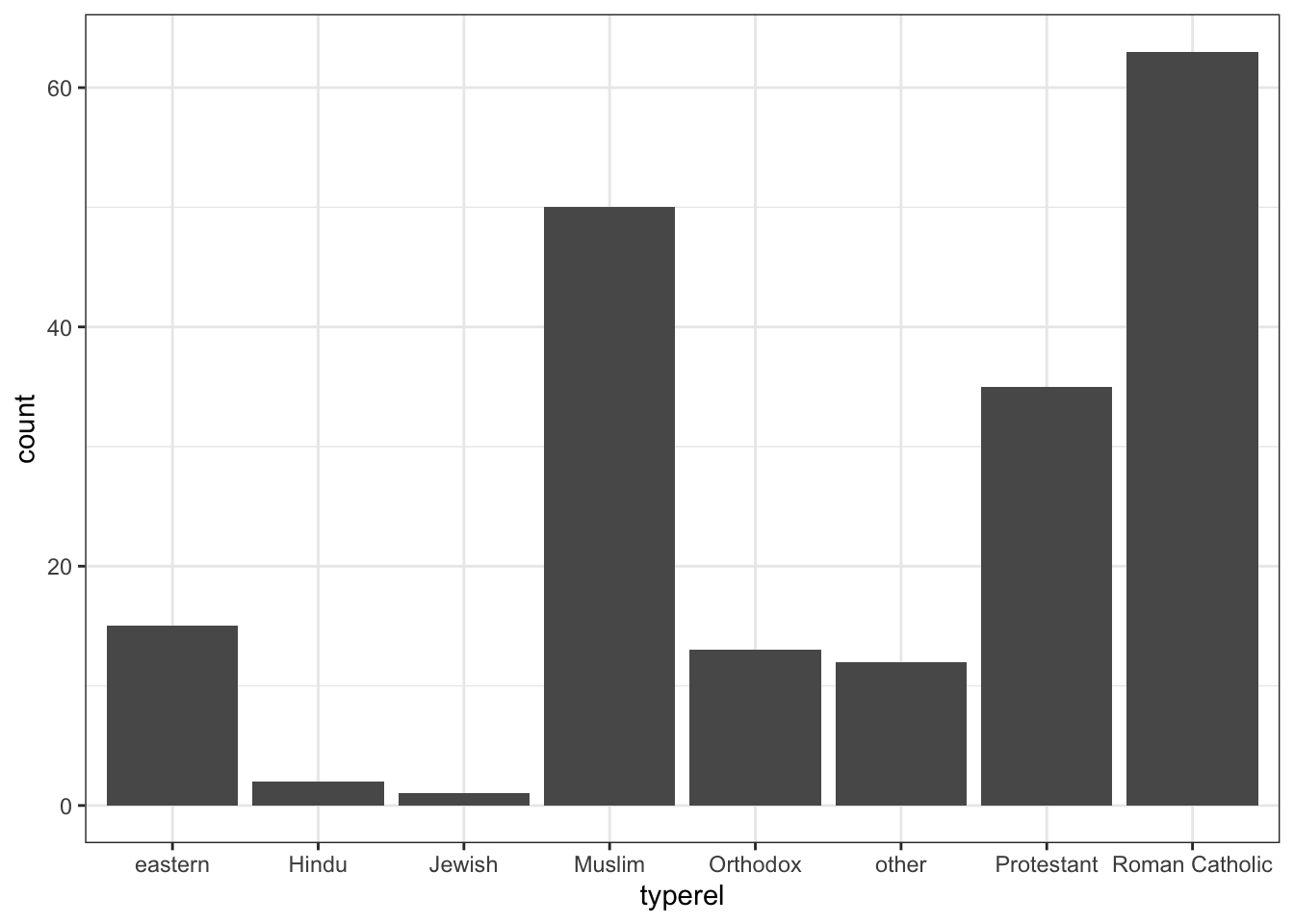
table( world.data $ typerel )
##
##        eastern          Hindu         Jewish         Muslim       Orthodox
##             15              2              1             50             13
##          other     Protestant Roman Catholic
##             12             35             63
Make this frequency table vertical using the data.frame function
data.frame( table( world.data $ typerel ) )
##             Var1 Freq
## 1        eastern   15
## 2          Hindu    2
## 3         Jewish    1
## 4         Muslim   50
## 5       Orthodox   13
## 6          other   12
## 7     Protestant   35
## 8 Roman Catholic   63
Create a frequency table for the typerel variable
ft.typerel <- data.frame( table(world.data $ typerel) )
ft.typerel $ Percent <- round(prop.table(ft.typerel $ Freq) * 100, digits = 2)
colnames(ft.typerel)[colnames(ft.typerel) == "Var1"] <- "Religion"
ft.typerel
##         Religion Freq Percent
## 1        eastern   15    7.85
## 2          Hindu    2    1.05
## 3         Jewish    1    0.52
## 4         Muslim   50   26.18
## 5       Orthodox   13    6.81
## 6          other   12    6.28
## 7     Protestant   35   18.32
## 8 Roman Catholic   63   32.98
Which religion is the most “popular” in the world? That is, what is the mode of the “typerel” variable?
Roman Catholic is the most popular
What is the percentage of countries where muslim is the majority?
26.18%
Create a frequency table for democ_regime
ft.dr <- data.frame( table(world.data $ democ_regime) )
ft.dr $ Percent <- round(prop.table(ft.dr $ Freq) * 100, digits = 2)
colnames(ft.dr)[colnames(ft.dr) == "Var1"] <- "Democracy?"
ft.dr
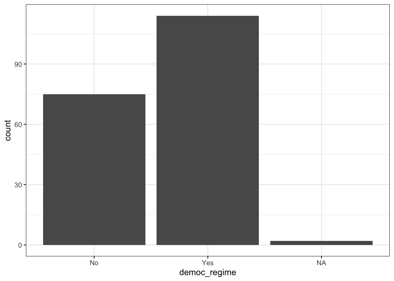
##   Democracy? Freq Percent
## 1         No   75   39.68
## 2        Yes  114   60.32
What percentage of countries have a democratic regime?
60.32%
Create a bar chart to summarize the typerel variable
ggplot(world.data, aes(x = typerel)) + geom_bar() + theme_bw()
Create a bar chart to summarize the democ_regime variable
ggplot(world.data, aes(x = democ_regime)) + geom_bar() + theme_bw()
3. Making ggplot graphs look nicer
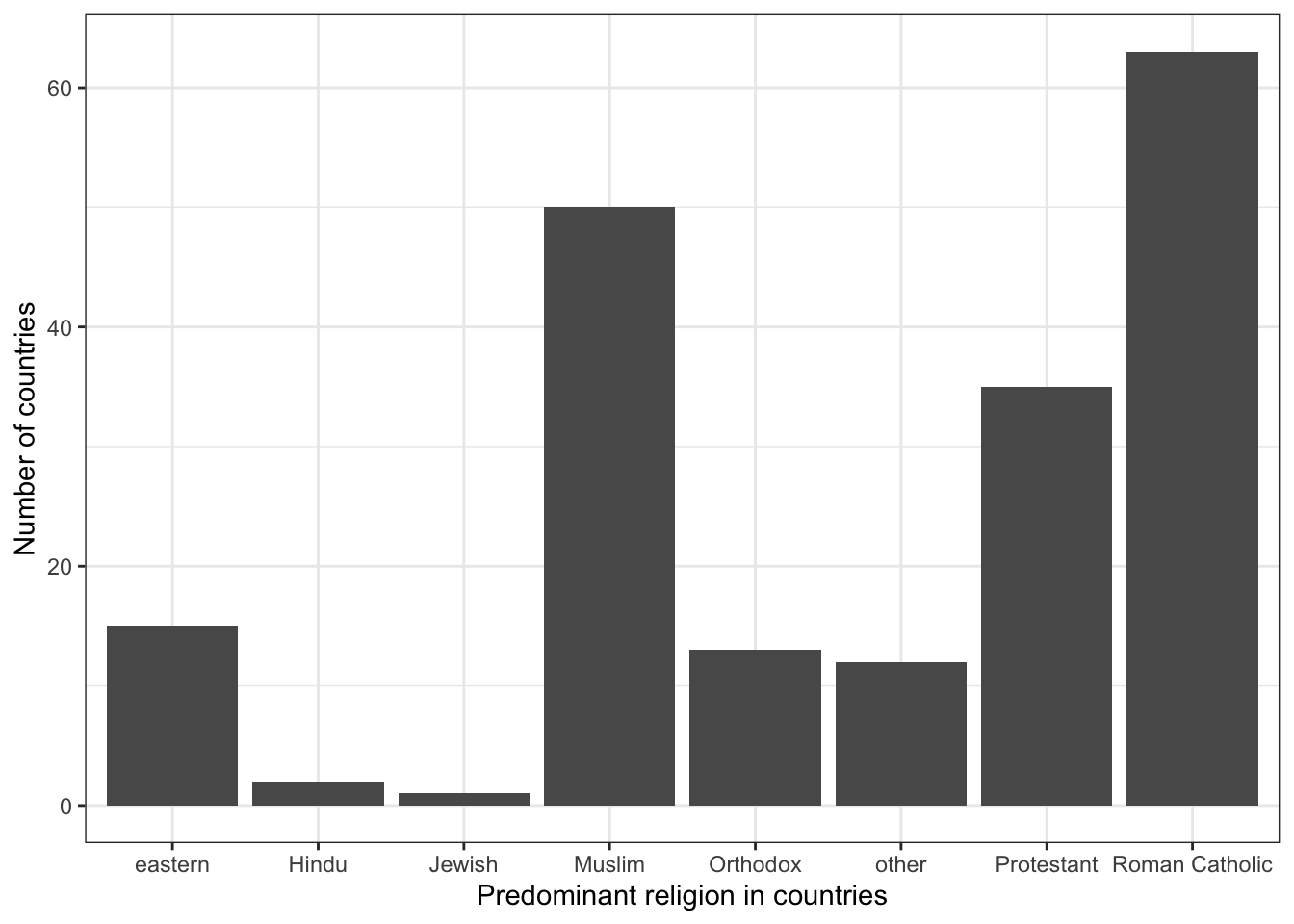
Create a bar chart for the typerel variable, and save it as a PDF file
g <- ggplot(world.data)
g <- g + aes(x = typerel)
g <- g + geom_bar()
g <- g + xlab("Predominant religion in countries")
g <- g + ylab("Number of countries")
g <- g + theme(axis.text.x = element_text(size = 12)) + theme_bw()
g
# ggsave(file = "religion_bar.pdf", width = 10, height = 8)
4. Summarizing numerical variables
Numerically summarize the gini04 variable.
That is, calculate and present the measures for central tendency and those for dispersion.
summary(world.data $ gini04)
##    Min. 1st Qu.  Median    Mean 3rd Qu.    Max.    NA's
##   24.40   32.42   37.95   40.14   46.88   70.70      65
sd(world.data $ gini08, na.rm = TRUE)
## [1] 9.999242
Numerically summarize the gini08 variable.
That is, calculate and present the measures for central tendency and those for dispersion.
summary(world.data $ gini08)
##    Min. 1st Qu.  Median    Mean 3rd Qu.    Max.    NA's
##   24.70   33.55   39.20   40.74   47.10   74.30      64
sd(world.data $ gini08, na.rm = TRUE)
## [1] 9.999242
Compare the distributions of gini04 and gini08.
Do you think that the level of economic inequality is getting worse, getting better, or neither? Why or why not?
Note: I’m not asking why it is getting better, worse, or neither; I’m asking on what basis you can conclude that it’s getting better or worse.
The level of economic inequality in the world seems to have deteriorated but only slightly. Although the quartile values of Gini coefficient got greater from 2004 to 2008, the mean value of Gini coefficient changed very little from 2004 and 2008 are very similar.
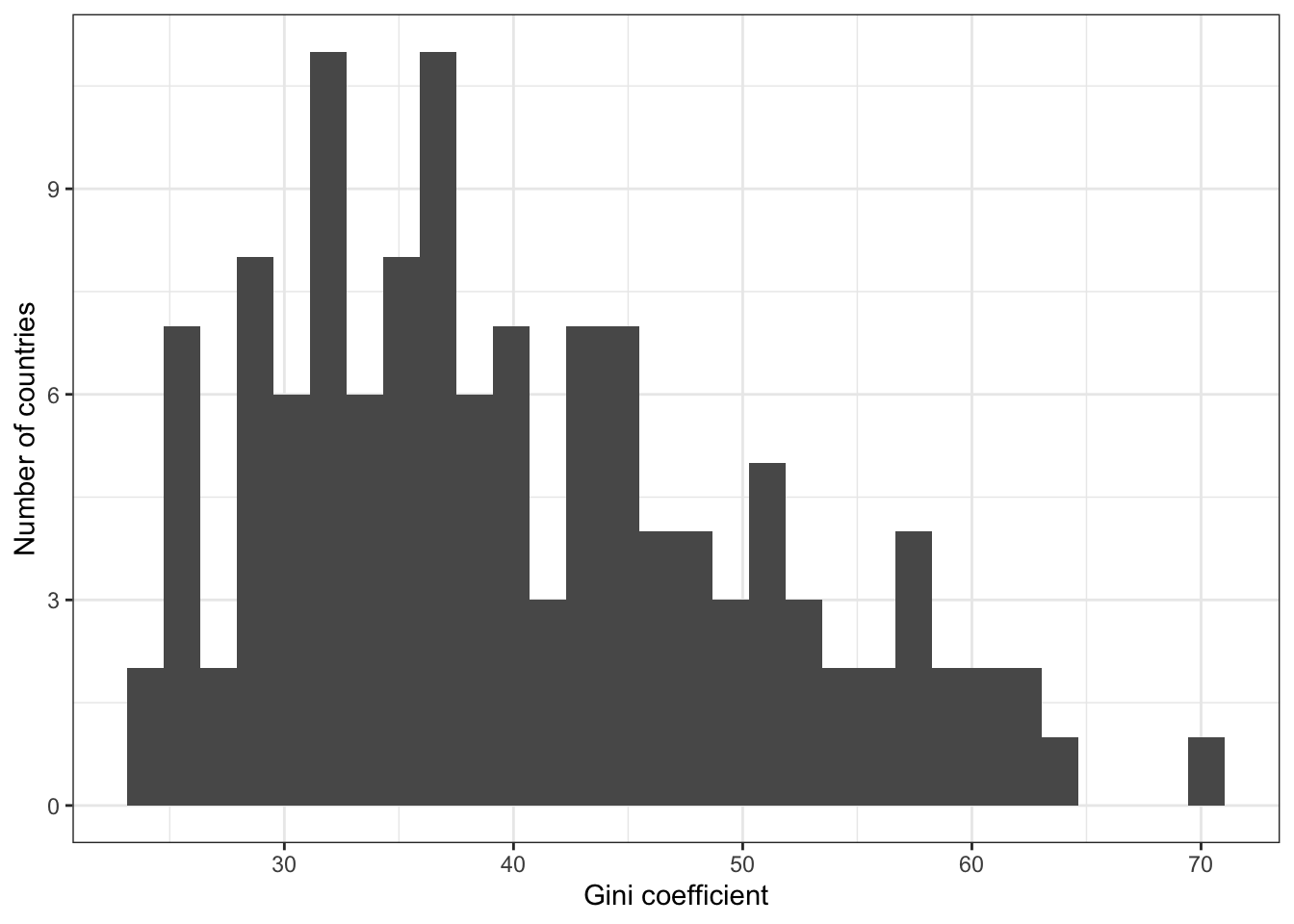
Create a histogram of gini04
Modify the axis labels accordingly to make them informative and intuitive. Save the graph as a PDF file.
g <- ggplot(world.data, aes(x = gini04))
g <- g + geom_histogram()
g <- g + theme(axis.text.x = element_text(size = 12))
g <- g + xlab("Gini coefficient")
g <- g + ylab("Number of countries") + theme_bw()
g
# ggsave(file = "gini04_hist.pdf", width = 10, height = 8)
Create a histogram of gini08
Modify the axis labels accordingly to make them informative and intuitive. Save the graph as a PDF file.
g<- ggplot(world.data, aes(x = gini08))
g <- g + geom_histogram()
g <- g + theme(axis.text.x = element_text(size = 12))
g <- g + xlab("Gini coefficient")
g <- g + ylab("Number of countries") + theme_bw()
g
# ggsave(file = "gini08_hist.pdf", width = 10, height = 8)
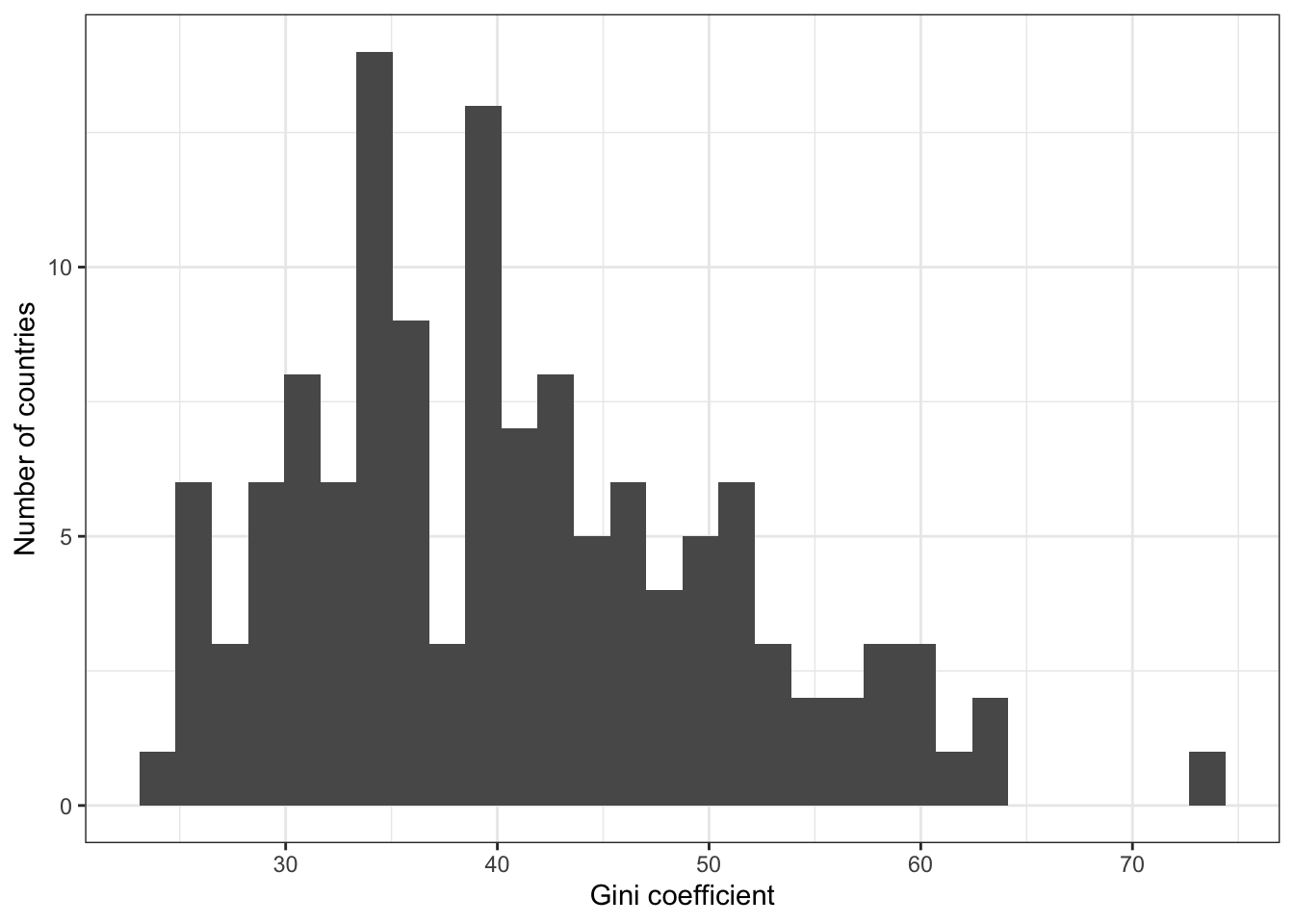
Compare the distributions of gini04 and gini08 graphically by placing the two PDF files you just created side by side.
Do you confirm the conclusion you derived previously?
Ans: The two histograms look very similar, which is consistent with the conclusion we derived above that the change was, if anything very subtle.
As we saw in the lecture, we sometimes create histograms for different values of a nominal-level variable. For example, we may want to create separate histograms of gini04 for countries in different regions.
How do we do it?
To do so, we use the facet_wrap option, as follows.
g <- ggplot(world.data, aes(x = gini04))
g <- g + geom_histogram()
g <- g + theme(axis.text.x = element_text(size = 12))
g <- g + xlab("Gini coefficient")
g <- g + ylab("Number of countries")
g <- g + facet_wrap( ~ region) + theme_bw()
g
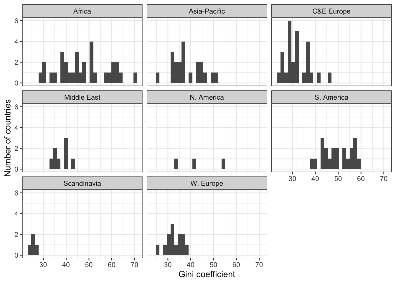
We can see that Scandinavian countries and Western European countries have, on average, lower Gini coefficients (= they are more egalitarian), whereas countries in South America have relatively high values.
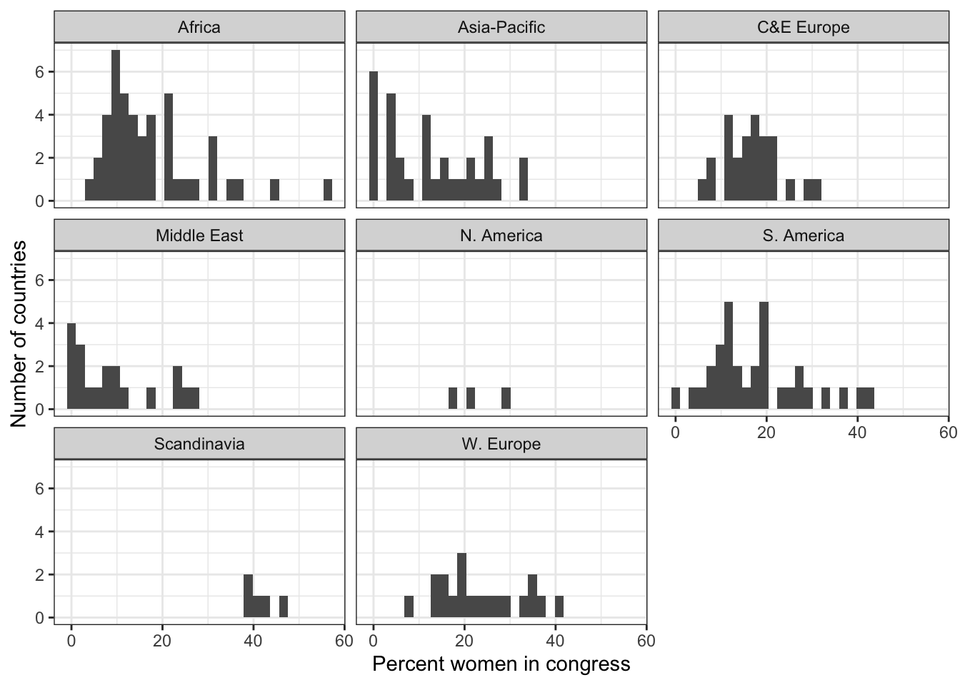
Create separate histograms of women09 for countries in different regions.
g <- ggplot(world.data, aes(x = women09))
g <- g + geom_histogram()
g <- g + theme(axis.text.x = element_text(size = 12))
g <- g + xlab("Percent women in congress")
g <- g + ylab("Number of countries")
g <- g + facet_wrap( ~ region) + theme_bw()
g
Calculate the standard deviation of gini04 for different regions using the by function
Hint: we still need to take care of the missing value problem.Use the na.rm = TRUE option.
by(world.data $ gini04, world.data $ region, sd, na.rm = TRUE)
## world.data$region: Africa
## [1] 11.06417
## ------------------------------------------------------------
## world.data$region: Asia-Pacific
## [1] 6.651417
## ------------------------------------------------------------
## world.data$region: C&E Europe
## [1] 5.167651
## ------------------------------------------------------------
## world.data$region: Middle East
## [1] 3.314901
## ------------------------------------------------------------
## world.data$region: N. America
## [1] 10.89327
## ------------------------------------------------------------
## world.data$region: S. America
## [1] 6.329504
## ------------------------------------------------------------
## world.data$region: Scandinavia
## [1] 0.9831921
## ------------------------------------------------------------
## world.data$region: W. Europe
## [1] 3.679761
Which region has the smallest dispersion?
Scandinavian countries have the smallest dispersion.